---
title: "G-Computation: The Causal Tool You Should Be Using After Regression"
description: "Why reading regression coefficients directly is rarely sufficient for decision-making, and how g-computation delivers the causal estimates that actually answer business questions. With full R implementation using marginaleffects."
date: 2026-09-28
categories: [causal inference, g-computation, R, marginaleffects]
#draft: true
---
```{r}
#| include: false
knitr::opts_chunk$set(
message = FALSE,
warning = FALSE,
fig.width = 7,
fig.height = 4.5
)
```
The loyalty programme team presents their quarterly results. The lead analyst points to a coefficient of 0.42 on programme enrolment, p-value below 0.001, and declares that the programme is working. The CFO leans back and asks the only question that matters: by how much did it improve retention? The analyst has no answer. The coefficient does not have one.
This failure is not about the analyst's competence. It is about a persistent mismatch between what regression models produce and what decisions require. A logistic regression coefficient of 0.42 lives on the log-odds scale, a metric that has no direct probability interpretation. Converting it to an odds ratio of 1.52 does not resolve this: an odds ratio is a ratio of ratios, and it still does not tell you how many customers were retained because of the programme. The number that answers the CFO's question is a probability difference, the average change in retention probability attributable to programme enrolment, expressed in percentage points. That quantity is what g-computation delivers.
In the first post, [What Is a Counterfactual?](https://joaovieira22.github.io/posts/What_is_counterfactual/what-is-counterfactual-index.html), we established that causal inference is a missing-data problem: every unit has two potential outcomes, but we observe only one. G-computation is the direct operationalisation of that insight. It takes the outcome model already sitting in your R session and uses it to predict both potential outcomes for every unit, then averages the difference.
## The Problem with Reading the Coefficient
Consider a binary outcome $Y$ (whether a customer renews), a binary treatment $D$ (programme enrolment), and a vector of covariates $X$ (age, tenure, prior spend). You fit a logistic regression:
$$\log\left(\frac{P(Y=1 \mid D, X)}{1 - P(Y=1 \mid D, X)}\right) = \beta_0 + \beta_1 D + \boldsymbol{\beta}_2^\top X$$
The coefficient $\hat{\beta}_1 = 0.42$ is reported as the effect. Three properties of this quantity make it insufficient for decision-making.
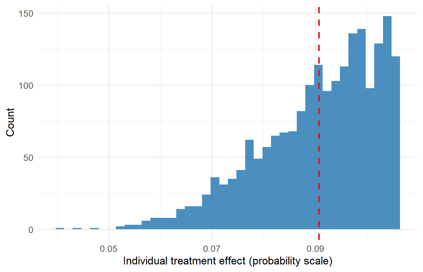
First, the coefficient lives on the log-odds scale. A change of 0.42 in log-odds has no direct probability interpretation without knowing the baseline. Second, the odds ratio $\exp(0.42) \approx 1.52$ exhibits non-collapsibility: it takes a different numerical value when computed conditional on different covariate sets, even in the complete absence of confounding. This is not a bias in the conventional sense, the conditional odds ratio is a consistent estimate of the conditional parameter, but it does mean that the odds ratio from a fully adjusted model is not directly comparable to one from a model with a different covariate set, nor does it aggregate cleanly to a marginal population summary. For resource allocation decisions, which require a single marginal effect interpretable across the population, this property limits comparability. Third, the marginal effect of $D$ on the probability scale varies across individuals. Because the logistic link is non-linear, a customer with a baseline renewal probability of 0.20 receives a different probability lift from the programme than one at 0.80. There is no single slope that summarises the treatment effect on the probability scale.
| Quantity | Value | Interpretable for a decision? |
|:---|:---:|:---|
| Coefficient (log-odds) | 0.42 | No |
| Odds ratio | 1.52 | Rarely: non-collapsibility limits population-level interpretation |
| Average treatment effect (probability) | 0.09 | Yes: 9 percentage points |
: Three ways to report the same model output. Only the third answers the CFO's question. {.striped}
The gap between 0.42 and 0.09 is not cosmetic. An organisation that makes resource allocation decisions based on log-odds coefficients is reporting on the wrong scale for the questions being asked. G-computation closes that gap by construction.
## Before Modelling: Causal Diagrams and Covariate Selection
G-computation is only as credible as the set of confounders it conditions on. Choosing those confounders is not a statistical question; it is a scientific one. The right tool for the job is a causal directed acyclic graph (DAG): a drawing of the assumed causal relationships between treatment, outcome, and background variables.
```{r}
#| label: dag
#| message: false
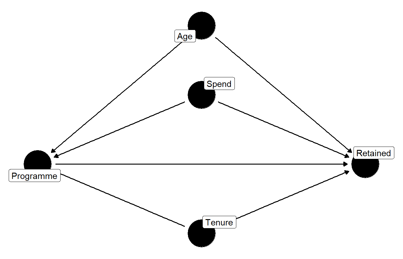
#| fig-cap: "A simple DAG for the loyalty programme example. Age, spend, and tenure each affect both programme enrolment and retention, making them confounders. The arrow from programme to retained is the causal path of interest. There is no unmeasured common cause (U), so the no-unmeasured-confounding assumption is satisfied by design in this simulated example."
library(ggdag)
library(ggplot2)

dag <- dagify(
  retained ~ programme + age + spend + tenure,
  programme ~ age + spend + tenure,
  coords = list(
    x = c(programme = 0, retained = 2, age = 1,
          spend = 1, tenure = 1),
    y = c(programme = 0, retained = 0, age = 1,
          spend = 0.5, tenure = -0.5)
  ),
  labels = c(
    retained  = "Retained",
    programme = "Programme",
    age       = "Age",
    spend     = "Spend",
    tenure    = "Tenure"
  )
)

ggdag(dag, use_labels = "label", text = FALSE) +
  theme_dag()
```
Reading the DAG identifies the **adjustment set**, the variables that must enter the outcome model to block all back-door paths from treatment to outcome. Here, age, spend, and tenure are confounders (they affect both enrolment and retention), so they must be included. A variable that is a collider or a mediator should generally be excluded; including it can introduce bias even when it improves model fit statistics. A useful heuristic: fit what the DAG says, not what the stepwise selector says.
::: {.callout-note}
## The adjustment set comes from science, not from software
Covariate selection for g-computation should begin with a DAG, not with a variable selection algorithm. Including a variable that is only a predictor of the outcome (a prognostic variable) is safe and improves precision. Including a collider biases the estimate. Including a mediator blocks the causal path you want to estimate. The `ggdag` and `dagitty` packages make it straightforward to enumerate valid adjustment sets programmatically via `dagitty::adjustmentSets()`.
:::
## The G-Formula: A Counterfactual Machine
G-computation, introduced by Robins (1986), is the direct operationalisation of the counterfactual framework. Under the standard identifiability assumptions, conditional exchangeability (no unmeasured confounders given $X$), positivity (every covariate stratum has both treated and untreated units), and consistency (the observed outcome equals the potential outcome under the assigned treatment), the average treatment effect is identified as:
$$\text{ATE} = E\bigl[E[Y \mid D=1, X] - E[Y \mid D=0, X]\bigr]$$
where the outer expectation averages over the marginal distribution of $X$. This is the g-formula. Estimation proceeds in three steps: fit an outcome model $\hat{E}[Y \mid D, X]$ on the observed data; generate two counterfactual predictions for every unit, one setting $D=1$ and one setting $D=0$, each with $X_i$ held at its observed value; then average the differences.
The reason this works in non-linear models is that $X_i$ is held fixed at each individual's observed values. You are comparing the same individual under two treatment states, the closest observational data gets to an individual causal effect.
For the Average Treatment Effect on the Treated (ATT), which asks what the programme did for the customers who actually enrolled:
$$\widehat{ATT} = \frac{1}{N_T} \sum_{i:\,D_i=1} \left[\hat{P}(Y=1 \mid D=1, X_i) - \hat{P}(Y=1 \mid D=0, X_i)\right]$$
::: {.callout-note}
## Identification depends on what you measured
G-computation is no more and no less assumption-dependent than any other regression-based causal method. The no-unmeasured-confounding assumption is untestable from data alone. What g-computation adds is transparency: it forces you to specify the outcome model explicitly, and it delivers the causal estimate on the outcome scale rather than the scale of the linear predictor.
:::
## Marginal Effects, Slopes, and Comparisons
The term "marginal" appears everywhere in the output of `marginaleffects`, marginal effects, marginal slopes, average marginal effects, marginal effects at the mean, and the terminology is notoriously slippery. This section pins down what each of these quantities actually is, how they relate to g-computation, and why the distinction between slopes and comparisons matters for binary treatments in non-linear models. The treatment here follows the framework laid out in Andrew Heiss's excellent guide to [Marginalia](https://www.andrewheiss.com/blog/2022/05/20/marginalia/).
### What Does "Marginal" Mean?
In statistics, "marginal" means "additional": what happens to the outcome $Y$ when an explanatory variable $X$ changes a little, holding everything else fixed. For a continuous predictor, this is a partial derivative, $\partial E[Y \mid X] / \partial X_k$, the instantaneous rate of change in the outcome associated with an infinitesimal increase in $X_k$. For a binary or categorical predictor, the change is discrete: you evaluate the model with the switch on and with the switch off, and take the difference. These are conceptually distinct operations, and the `marginaleffects` package separates them into two families of functions: `slopes()` for derivatives (continuous sliders) and `comparisons()` for discrete contrasts (categorical switches).
### Sliders and Switches
A useful analogy, due to Heiss, is to think of regression predictors as sliders and switches on a mixing board. Continuous variables are sliders: as you move them up and down, the outcome changes gradually, and the marginal effect is the slope of that change, the tangent to the response curve at a given setting. Categorical variables are switches: they are either on or off, and the marginal effect is the difference in the outcome between two switch positions. You cannot talk about a one-unit increase in "programme-ness" any more than you can talk about the derivative of a light switch.
In a linear model with no interactions, the slider slope is constant everywhere and the switch difference is the same for every unit, so the coefficient table already contains the marginal effects. In a non-linear model, logistic, Poisson, negative binomial, Cox, both quantities vary across individuals because the response curve is non-linear. The coefficient alone is no longer sufficient, and we need to compute marginal effects after fitting the model.
### Average Marginal Effects (AME) vs. Marginal Effects at the Mean (MEM)
Once we accept that marginal effects vary across units, the next question is how to summarise them into a single number. Two approaches dominate the literature, and they produce different results in non-linear models because they average in a different order.
The **average marginal effect (AME)** is the default in `marginaleffects`. It computes a marginal effect, slope or comparison, for each observation in the dataset, using that observation's actual covariate values, and then averages across all observations. Formally, for a continuous predictor $X_k$:
$$\text{AME}_k = \frac{1}{n}\sum_{i=1}^{n} \frac{\partial E[Y \mid X_i]}{\partial X_{ik}}$$
Each term in the sum uses real, observed covariate values. The AME reflects the distribution of covariates in the sample, which makes it representative of the population in the data. Because it averages many observations, its standard error is typically smaller than that of the MEM.
The **marginal effect at the mean (MEM)** averages the covariates first, then computes the marginal effect at that single point. It plugs in $\bar{X}$ and evaluates the slope or comparison there:
$$\text{MEM}_k = \frac{\partial E[Y \mid X = \bar{X}]}{\partial X_k}$$
No actual observation may have covariate values equal to $\bar{X}$. The MEM reflects a hypothetical "average unit" that might not exist in the data. In a linear model, AME and MEM coincide because the slope is constant; in a non-linear model, they generally differ, and the difference can be substantively meaningful, particularly when the response curve is steep near the mean or when the covariate distribution is skewed.
In `marginaleffects`, the AME is the default: `avg_slopes(mod)` or `avg_comparisons(mod)` averages over the original data. The MEM is obtained by setting `newdata = "mean"`. The `emmeans` package reverses this convention: `emtrends()` computes the MEM by default. This difference in defaults has caused considerable confusion in practice; the numerical results are not directly comparable across packages unless the averaging convention is matched.
### Slopes (Continuous Predictors) vs. Comparisons (Binary Predictors)
For a continuous predictor, the natural marginal quantity is the partial derivative, the slope of the response surface with respect to that predictor. `avg_slopes()` computes this. For a binary predictor, the natural quantity is the discrete contrast: the difference in predicted outcomes when the variable is set to 1 versus 0. `avg_comparisons()` computes this. In a linear model the two coincide, because the derivative is constant and equals the discrete difference. In a non-linear model they diverge, and the divergence is not a software artefact, it reflects a genuine conceptual mismatch between an infinitesimal approximation and the estimation of a discrete jump.
Formally, for a logistic model with coefficient $\hat{\beta}_1$ on the binary treatment, `avg_comparisons()` computes:
$$\frac{1}{n}\sum_{i=1}^{n}\Bigl[\sigma(\hat{\beta}_0 + \hat{\beta}_1 + X_i^\top\hat{\boldsymbol{\beta}}_2) - \sigma(\hat{\beta}_0 + X_i^\top\hat{\boldsymbol{\beta}}_2)\Bigr]$$
where $\sigma(\cdot) = \text{logit}^{-1}(\cdot)$. This is the g-computation ATE: the average difference in predicted probabilities between the two counterfactual treatment states. The partial derivative that `avg_slopes()` would compute for the same binary variable is:
$$\frac{1}{n}\sum_{i=1}^{n} \hat{\beta}_1 \cdot \hat{p}_i \bigl(1 - \hat{p}_i\bigr)$$
where $\hat{p}_i = \sigma(\hat{\eta}_i)$ is the fitted probability at the **observed** treatment value $D_i$ for unit $i$. These are different quantities. The first is a discrete counterfactual contrast; the second is an average of local tangent slopes. Because the logistic curve is S-shaped, the derivative is largest near the midpoint ($p = 0.5$) and attenuated near the tails: treated units with high predicted probabilities have small slopes, which drags the average derivative below the discrete comparison. The derivative approximates what the comparison would return for a continuous predictor but does not correspond to a discrete counterfactual contrast.
### Why `avg_slopes()` and `avg_comparisons()` Return the Same Number for Binary Variables
Recent versions of `marginaleffects` (0.20.0 and later) auto-detect binary and categorical variables and convert `avg_slopes()` calls into discrete comparisons, matching `avg_comparisons()` output. This is a sensible software default, computing a derivative for a binary variable is rarely what the analyst intends, but it means that calling `avg_slopes()` on a binary treatment no longer reveals the conceptual difference between the two quantities. Under the hood, the package recognises that the variable is not a slider and substitutes a switch operation.
To see that the underlying quantities genuinely differ, we compute the derivative manually and compare it with the discrete comparison:
```{r}
#| label: comparisons-vs-slopes
library(marginaleffects)

set.seed(101)
n <- 1000
demo <- data.frame(
  x = rnorm(n),
  d = rbinom(n, 1, 0.5)
)
demo$y <- rbinom(n, 1, plogis(-0.5 + 2 * demo$d + 0.4 * demo$x))

mod_bin <- glm(y ~ d + x, data = demo, family = binomial)

# avg_comparisons(): discrete 0→1 contrast (the g-computation ATE)
cat("avg_comparisons() [discrete 0→1]:  ",
    round(avg_comparisons(mod_bin, variables = "d")$estimate, 4), "\n")
# avg_slopes() on a binary variable: auto-converted to a comparison,
# so it matches avg_comparisons() by design
cat("avg_slopes()     [auto-converted]:  ",
    round(avg_slopes(mod_bin, variables = "d")$estimate, 4), "\n")
# Manual derivative: what avg_slopes() *would* compute without auto-conversion
#   dp/dD = beta_D * p * (1 - p), evaluated at each unit's observed D
p_obs  <- predict(mod_bin, type = "response")
beta_d <- coef(mod_bin)["d"]
derivs <- beta_d * p_obs * (1 - p_obs)

cat("Average derivative at observed D:   ",
    round(mean(derivs), 4), "\n")
```
The `avg_comparisons()` result is the average risk difference associated with moving from $D=0$ to $D=1$, the g-computation ATE on the probability scale. The average derivative is the weighted average of unit-level tangent slopes, evaluated at each observation's own value of $D$; it is the appropriate quantity for a continuous predictor but a less suitable one for a discrete treatment. Because the logistic curve is S-shaped, the derivative is largest near the midpoint and attenuated near the tails: treated units with high predicted probabilities have small slopes, which drags the average derivative below the discrete comparison. In settings where the treatment coefficient is large or where treated units cluster near the tails of the predicted probability distribution, the difference between the two quantities can be substantively meaningful.
::: {.callout-warning}
## Use `avg_comparisons()` for binary treatments, `avg_slopes()` for continuous predictors
For a binary or categorical treatment in a logistic, Poisson, negative binomial, or Cox model, always use `avg_comparisons()`. It evaluates the model at two discrete treatment levels and takes the difference. `avg_slopes()` is designed for continuous predictors: it computes a derivative assuming infinitesimal variation in the focal variable. In recent `marginaleffects` versions, calling `avg_slopes()` on a binary variable auto-converts to a comparison, hiding the conceptual distinction.
:::
## ATE, ATT, and ATU: Choosing Your Estimand
The choice of estimand is a research design decision that precedes any modelling. It follows directly from the policy question, not from computational convenience. G-computation makes this choice transparent: the estimand is determined by which units' covariate profiles you average the counterfactual predictions over.
The **ATE** averages over the full sample. It answers: if we applied the treatment to a randomly selected individual from the population, what is the expected effect? This is appropriate when the question is whether to introduce a programme universally.
The **ATT** averages only over units that received the treatment. It answers: what did the programme do for the participants? This is the natural choice for retrospective evaluation of an existing programme.
The **ATU** averages over units that did not receive treatment. It answers: what would the programme do for the non-participants if we extended it to them? This is the right estimand when the decision is whether to scale up a pilot.
In `marginaleffects`, the estimand is controlled by the `newdata` argument of `avg_comparisons()`.
| Policy question | Estimand | `newdata` argument |
|:---|:---|:---|
| Did the programme work for participants? | ATT | `subset(dat, D == 1)` |
| Should we roll this out to everyone? | ATE | `NULL` (default) |
| Should we extend it to non-participants? | ATU | `subset(dat, D == 0)` |
: Estimand selection. The choice is substantive, not technical, and should be made before fitting the model. {.striped}
```{r}
#| label: estimands
dat_lot <- get_dataset("lottery")
dat_lot <- subset(dat_lot, win_big == 1 | win == 0)

mod_lot <- lm(
  earnings_post_avg ~ win_big * (tickets + man + work + age +
    education + college + year +
    earnings_pre_1 + earnings_pre_2 + earnings_pre_3),
  data = dat_lot
)

ate <- avg_comparisons(mod_lot, variables = "win_big")
att <- avg_comparisons(mod_lot, variables = "win_big",
                       newdata = subset(dat_lot, win_big == 1))
atu <- avg_comparisons(mod_lot, variables = "win_big",
                       newdata = subset(dat_lot, win_big == 0))

cat("ATE:", round(ate$estimate, 2), "\n")
cat("ATT:", round(att$estimate, 2), "\n")
cat("ATU:", round(atu$estimate, 2), "\n")
```
The ATT and ATU generally differ when treatment effects are heterogeneous and when selection into treatment is not random. In the lottery example, people who buy more tickets have different baseline earnings profiles from those who buy fewer; winning a large prize has a different effect on their subsequent labour supply. The ATE averages over both groups and may describe neither well. Reporting all three estimands takes three lines of code and substantially improves the decision-relevance of the output.
::: {.callout-tip}
## Which estimand to report
In most business settings, the ATT is the natural starting point: did the programme work for the people who enrolled? If yes, the next question is whether to extend it, which requires the ATU. The ATE is appropriate when the question is whether to introduce a programme from scratch across an entire population. Always state which estimand you are reporting, because the same word "effect" can refer to any of the three.
:::
## G-Computation Across Model Types
One of the practical strengths of g-computation is that the procedure is identical regardless of the model type: fit the model, predict under each counterfactual, average the difference. What changes across model families is the scale of the outcome and, consequently, the interpretation of the effect.
### Binary Outcome: Logistic Regression
For a binary outcome the g-computation estimate is a risk difference, the average change in the probability of the event. This is the quantity that translates directly into a count of additional customers retained, conversions achieved, or defaults avoided.
```{r}
#| label: logistic-gcomp
#| fig-cap: "Distribution of unit-level treatment effects across the sample. Because the logistic curve is non-linear, the effect varies across individuals, the coefficient table collapses this variation into a single number that may not represent any individual well."
library(ggplot2)
library(marginaleffects)

set.seed(42)
n <- 2000
loyalty <- data.frame(
  age       = rnorm(n, 45, 12),
  spend     = rnorm(n, 500, 200),
  tenure    = rnorm(n, 3, 1.5),
  programme = rbinom(n, 1, 0.4)
)
loyalty$prob <- plogis(-1.5 + 0.3 * loyalty$programme +
                       0.02 * loyalty$age - 0.001 * loyalty$spend +
                       0.1  * loyalty$tenure)
loyalty$retained <- rbinom(n, 1, loyalty$prob)

mod_logit <- glm(retained ~ programme + age + spend + tenure,
                 data = loyalty, family = binomial)

# Unit-level counterfactual predictions via marginaleffects::predictions()
p1 <- predictions(mod_logit,
                  newdata = transform(loyalty, programme = 1))
p0 <- predictions(mod_logit,
                  newdata = transform(loyalty, programme = 0))

unit_effects <- p1$estimate - p0$estimate

ggplot(data.frame(effect = unit_effects), aes(x = effect)) +
  geom_histogram(bins = 40, fill = "#2c7bb6", alpha = 0.85) +
  geom_vline(xintercept = mean(unit_effects), colour = "#d7191c",
             linetype = "dashed", linewidth = 1) +
  labs(x = "Individual treatment effect (probability scale)",
       y = "Count") +
  theme_minimal(base_size = 13)
```
```{r}
# ATT in probability units
att_logit <- avg_comparisons(mod_logit, variables = "programme",
                             newdata = subset(loyalty, programme == 1))
print(att_logit)
```
::: {.callout-tip}
## Reporting recommendation: binary outcome
Report the ATT as a percentage point change with a 95% confidence interval: "Programme enrolment increased 12-month retention by X percentage points among enrolled customers (95% CI: a to b pp)." Include the baseline predicted probability under control to give the percentage point figure context. The logistic coefficient and odds ratio belong in the technical appendix.
:::
### Exploring Heterogeneity with CATE
Beyond the average effect, analysts often need to know *for whom* the treatment works best. The Conditional Average Treatment Effect (CATE) conditions on a subgroup variable. `plot_comparisons()` from the `marginaleffects` package makes this straightforward.
```{r}
#| label: cate
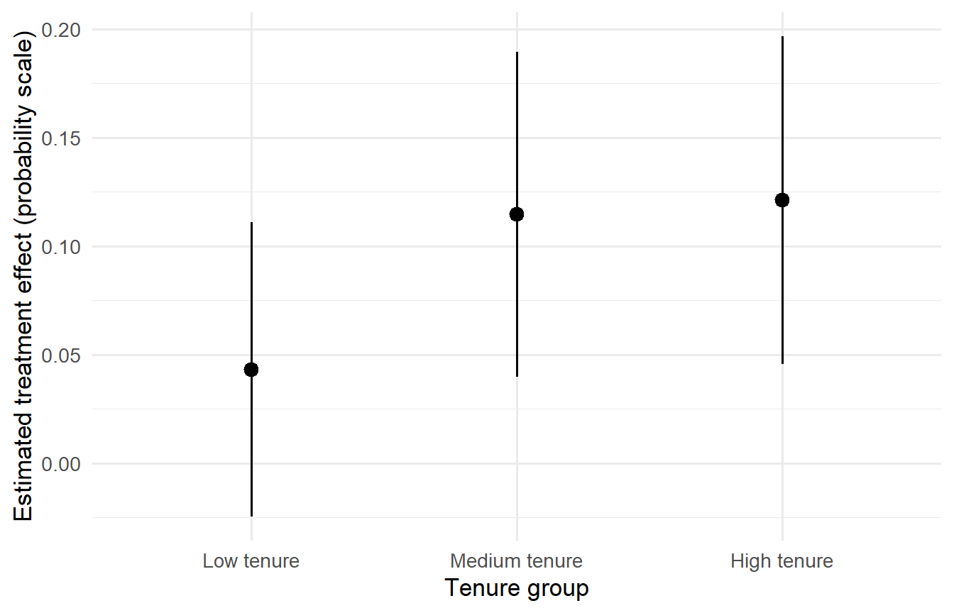
#| fig-cap: "Conditional average treatment effect by tenure group, estimated from a model with a programme × tenure_group interaction. The programme has a larger retention effect among long-tenured customers; among recent acquisitions it is close to zero."
loyalty$tenure_group <- cut(
  loyalty$tenure,
  breaks = quantile(loyalty$tenure, probs = c(0, 1/3, 2/3, 1)),
  labels = c("Low tenure", "Medium tenure", "High tenure"),
  include.lowest = TRUE
)

mod_cate <- glm(
  retained ~ programme * tenure_group + age + spend,
  data = loyalty, family = binomial
)

plot_comparisons(
  mod_cate,
  variables = "programme",
  condition = "tenure_group"
) +
  labs(x = "Tenure group",
       y = "Estimated treatment effect (probability scale)") +
  theme_minimal(base_size = 13)
```
These subgroup estimates can guide targeting: if the CATE is near zero for low-tenure customers but large for high-tenure ones, extending the programme to new customers allocates budget inefficiently. The subgroup ATT with confidence intervals is one additional `avg_comparisons()` call away:
```{r}
#| label: cate-by-group
#| eval: false
avg_comparisons(mod_cate, variables = "programme",
                newdata = subset(loyalty, tenure_group == "High tenure"))
```
### Count Outcome: Negative Binomial Regression
When the outcome is a non-negative integer, certifications completed, support tickets opened, products purchased, a Poisson or negative binomial model is appropriate, the latter handling overdispersion. The exponentiated coefficient is an Incidence Rate Ratio (IRR): a multiplicative factor on the rate. For operational decisions, how many additional certifications per employee to expect if training is extended, an absolute count difference is more directly actionable.
```{r}
#| label: nb-gcomp
library(MASS)
library(marginaleffects)

set.seed(123)
n2     <- 1500
trdata <- data.frame(
  experience = rnorm(n2, 5, 2),
  dept_size  = rpois(n2, 20),
  programme  = rbinom(n2, 1, 0.35)
)
trdata$rate  <- exp(0.5 + 0.25 * trdata$programme +
                    0.1  * trdata$experience + 0.01 * trdata$dept_size)
trdata$certs <- rnegbin(n2, mu = trdata$rate, theta = 2)

mod_nb <- glm.nb(certs ~ programme + experience + dept_size,
                 data = trdata)

cat("IRR:", round(exp(coef(mod_nb)["programme"]), 3), "\n")
att_nb <- avg_comparisons(mod_nb, variables = "programme",
                          newdata = subset(trdata, programme == 1))
print(att_nb)
```
The IRR tells you the multiplicative factor; the g-computation estimate tells you the absolute expected difference in counts per participant. If the ATT is 0.8 additional certifications per employee per year and the programme covers 5,000 employees, the total expected impact is 4,000 additional certifications annually. The IRR of 1.35 does not give you that number without knowing the baseline rate.
::: {.callout-tip}
## Reporting recommendation: count outcome
Report both the absolute count difference from `avg_comparisons()` and the IRR from `exp(coef())`. The count difference drives the cost-benefit analysis; the IRR provides the relative effect for comparison with other studies. If you can report only one, report the count difference.
:::
### Time-to-Event: Cox Proportional Hazards
For time-to-event outcomes the standard model is the Cox proportional hazards model, and the default output is a hazard ratio. Hernán (2010) showed that the hazard ratio is a difficult quantity to interpret causally: because the risk set changes over follow-up as individuals experience the event, the subpopulations being compared at later time points are no longer exchangeable even in a randomised trial. The hazard ratio conflates the treatment effect with the differential depletion of susceptible individuals from each arm, making its causal interpretation problematic rather than straightforwardly invalid. These concerns apply with particular force when the treatment effect is not constant over time.
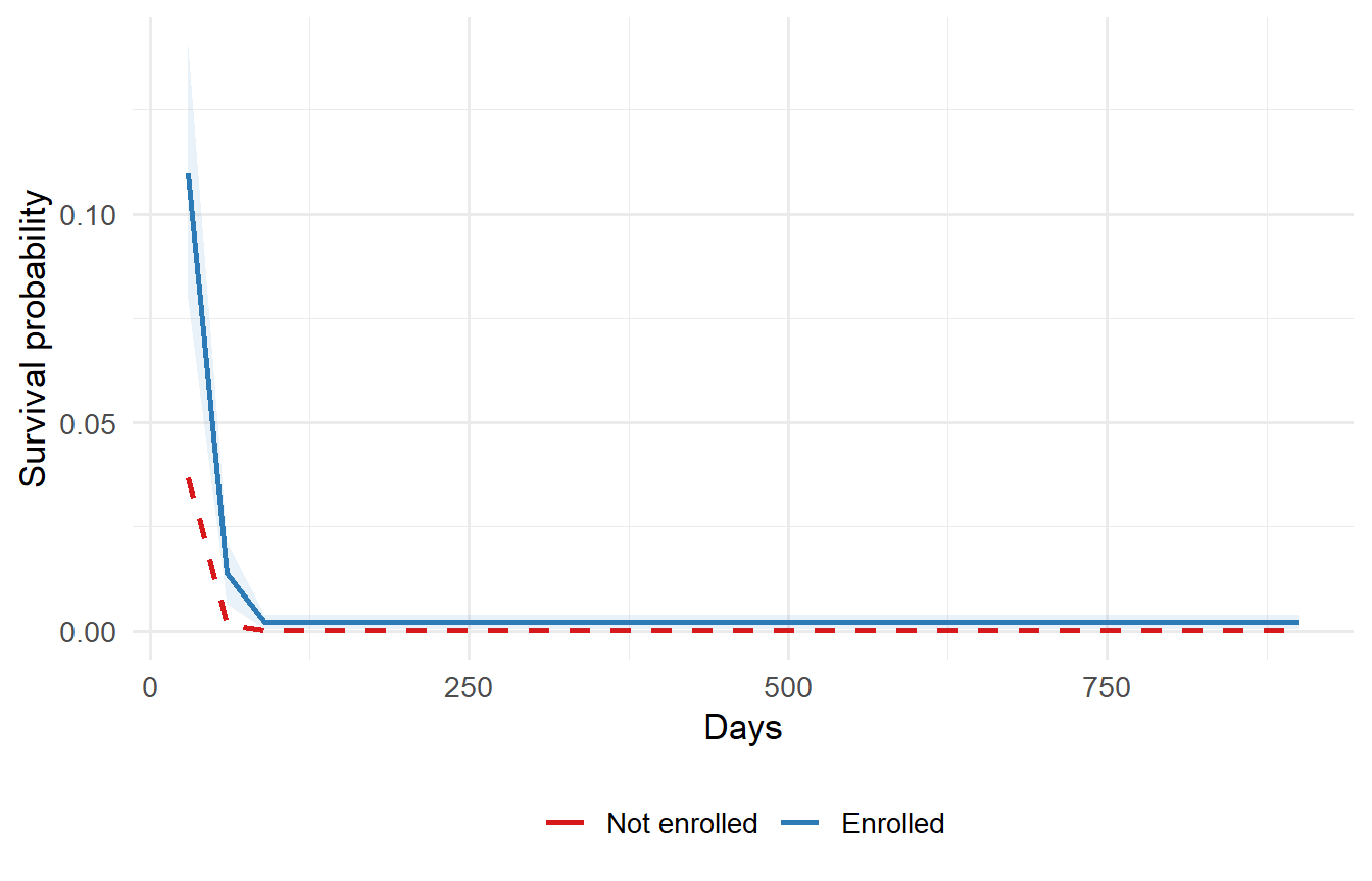
The more interpretable reporting quantity is the difference in marginalised survival probabilities at operationally meaningful time points. Because the baseline cumulative hazard $\hat{H}_0(t)$ is estimated non-parametrically by Breslow's estimator, the delta method does not capture its uncertainty reliably; bootstrap inference is required via `inferences()`.
```{r}
#| label: cox-gcomp
#| cache: true
#| fig-cap: "Marginalised survival curves under programme enrolment (blue, solid) and no enrolment (red, dashed). Each curve is the average of individual-level survival predictions across the observed covariate distribution. The gap at any time point is the g-computation estimate of the treatment effect at that horizon."
library(survival)
library(marginaleffects)
library(ggplot2)

set.seed(456)
n3 <- 1200
surv_dat <- data.frame(
  age3    = rnorm(n3, 50, 12),
  treated = rbinom(n3, 1, 0.5)
)
surv_dat$time  <- rexp(n3,
  rate = exp(-3 + (-0.5) * surv_dat$treated + 0.02 * surv_dat$age3))
surv_dat$event <- rbinom(n3, 1, 0.85)

mod_cox <- coxph(Surv(time, event) ~ treated + age3,
                 data = surv_dat, x = TRUE)

# Survival probability difference at 365 and 730 days
# Bootstrap via inferences() is required for Cox models
surv_comp <- avg_comparisons(
  mod_cox,
  variables = list(treated = c(0, 1)),
  type      = "survival",
  newdata   = datagrid(
    time    = c(365, 730),
    treated = 0:1,
    age3    = mean(surv_dat$age3),
    grid_type = "counterfactual"
  ),
  by = "time"
) |>
  inferences(method = "boot", R = 300)
print(surv_comp)
# Marginalised survival curves for plot
plot_grid <- expand.grid(
  time    = seq(30, 900, by = 30),
  treated = c(0, 1),
  age3    = mean(surv_dat$age3),
  event   = 1
)
plot_preds <- predictions(mod_cox, newdata = plot_grid, type = "survival")

ggplot(plot_preds, aes(x = time, y = estimate,
                       colour = factor(treated),
                       linetype = factor(treated))) +
  geom_line(linewidth = 0.9) +
  geom_ribbon(aes(ymin = conf.low, ymax = conf.high,
                  fill = factor(treated)),
              alpha = 0.1, colour = NA) +
  scale_colour_manual(values = c("0" = "#d7191c", "1" = "#2c7bb6"),
                      labels = c("Not enrolled", "Enrolled")) +
  scale_fill_manual(values = c("0" = "#d7191c", "1" = "#2c7bb6"),
                    guide = "none") +
  scale_linetype_manual(values = c("0" = "dashed", "1" = "solid"),
                        guide = "none") +
  labs(x = "Days", y = "Survival probability", colour = NULL) +
  theme_minimal(base_size = 13) +
  theme(legend.position = "bottom")
```
::: {.callout-warning}
## Cox models require bootstrap inference for survival curve differences
The baseline cumulative hazard $\hat{H}_0(t)$ in a Cox model is estimated separately from the regression coefficients by Breslow's estimator. Because it is non-parametric, the first-order Taylor approximation underlying the delta method does not account for its uncertainty. Confidence intervals based on the delta method for survival curve differences from Cox models will be too narrow. Always pipe through `inferences(method = "boot", R = ...)` for this type of quantity.
:::
::: {.callout-tip}
## Reporting recommendation: time-to-event
Report the difference in marginalised survival probabilities at pre-specified time points with bootstrap confidence intervals: "At 12 months, programme enrolment increased the probability of event-free survival by X percentage points (bootstrap 95% CI: a to b pp)." For non-technical audiences, the hazard ratio should be moved to the technical appendix; the causal interpretation difficulties noted above make it poorly suited as the primary reported quantity.
:::
## Uncertainty: Delta Method vs Bootstrap
Every g-computation estimate is a function of model parameters, and its uncertainty must be propagated accordingly. The `marginaleffects` package provides two main routes.
The delta method is the default. It propagates parameter uncertainty through the g-computation formula using a first-order Taylor approximation: if the ATE is a function $g(\hat{\boldsymbol{\beta}})$ of the coefficient vector, then
$$\widehat{\text{Var}}\bigl[g(\hat{\boldsymbol{\beta}})\bigr] \approx \nabla g(\hat{\boldsymbol{\beta}})^\top \, \hat{\Sigma} \, \nabla g(\hat{\boldsymbol{\beta}})$$
where $\hat{\Sigma}$ is the estimated coefficient covariance matrix and $\nabla g$ is the gradient. This is fast, analytically tractable, and valid for standard GLMs, logistic, Poisson, negative binomial, where the link function is smooth and the sample size is adequate.
The bootstrap is necessary when the delta method's first-order approximation is unreliable. The three main cases are: Cox models (because $\hat{H}_0(t)$ is non-parametric and the delta method does not account for its uncertainty); GAMs with complex spline terms (where the effective degrees of freedom are themselves estimated); and any highly non-linear derived quantity such as a ratio of two ATTs or an effect evaluated at a specific percentile of the covariate distribution.
```{r}
#| label: uncertainty-demo
#| eval: false
library(marginaleffects)

# Delta method (default), fast, valid for GLMs
avg_comparisons(mod_logit, variables = "programme")

# Heteroskedasticity-robust sandwich variance (HC3)
avg_comparisons(mod_logit, variables = "programme", vcov = "HC3")

# Bootstrap via inferences() wrapper, works for all model types
avg_comparisons(mod_logit, variables = "programme") |>
  inferences(method = "boot", R = 500)

# rsample-based bootstrap, integrates with tidymodels
avg_comparisons(mod_logit, variables = "programme") |>
  inferences(method = "rsample", R = 500)
```
For Cox models with survival outcomes, always use one of the bootstrap options above. A few hundred replicates suffice for exploratory work; 1,000 or more are standard for publication.
::: {.callout-note}
## When HC3 is appropriate
HC3 heteroskedasticity-robust standard errors are appropriate when the model may be somewhat misspecified, the normal condition for observational data. For logistic regression, variance heterogeneity is a structural feature of the model (binary outcomes are inherently more variable near $p = 0.5$), so HC3 is a sensible default for cross-sectional analyses. It is faster than the bootstrap and conservative rather than anti-conservative.
:::
## A Critical Limitation: Sensitivity to Model Misspecification
G-computation is statistically efficient; it extracts the maximum information from the outcome model. But it is heavily reliant on that model being correctly specified. If the functional form of $E[Y \mid D, X]$ is wrong, the g-computation estimate is inconsistent, it converges to the wrong answer even with infinite data. This is the price of efficiency.
The most common forms of misspecification in practice are: omitting interactions between treatment and covariates (which forces a homogeneous treatment effect when the truth is heterogeneous), missing non-linear covariate terms, and using a logistic model when the true relationship is more flexible. None of these can be detected from the data alone without additional assumptions.
Two practical responses are worth building into any analysis. First, compare the parametric g-formula prediction against the non-parametric observed mean within each treatment arm. Large discrepancies are informative warning signs, though agreement does not guarantee correct specification. Second, consider a doubly robust estimator that combines an outcome model with a propensity score model. A doubly robust estimator is consistent if *either* model is correctly specified, providing insurance against outcome model misspecification. The next post in this series introduces doubly robust estimation.
```{r}
#| label: natural-course-check
#| fig-cap: "A simple model check: the parametric natural-course mean (model predictions under observed treatment) versus the non-parametric observed mean. Close agreement is consistent with adequate model fit; large discrepancies indicate misspecification."
library(marginaleffects)

nc_pred <- mean(predictions(mod_logit)$estimate)
nc_obs  <- mean(loyalty$retained)

cat("Parametric natural-course mean:", round(nc_pred, 4), "\n")
cat("Observed mean: ", round(nc_obs, 4), "\n")
cat("Difference: ", round(nc_pred - nc_obs, 4), "\n")
```
::: {.callout-warning}
## G-computation is only as good as its outcome model
If the outcome model is misspecified, wrong functional form, missing interactions, omitted confounders, the g-computation estimate will be biased, and there is no statistical test that fully diagnoses this from the data alone. The natural-course check above is a necessary but not sufficient condition for model adequacy: a model can pass this check while still being misspecified in ways that distort the treatment effect estimate. When in doubt, pair g-computation with a doubly robust estimator.
:::
## The `marginaleffects` Ecosystem
`avg_comparisons()` is compatible with over 100 model classes in R. The table below summarises the most common in causal analysis work, with notes on when bootstrap inference is required.
| Model type | R function | Package | Bootstrap needed? |
|:---|:---|:---|:---|
| Linear regression | `lm()` | stats | No |
| Logistic / GLM family | `glm()` | stats | No |
| Negative binomial | `glm.nb()` | MASS | No |
| Generalised additive model | `gam()` | mgcv | Recommended for complex smooths |
| Cox proportional hazards | `coxph()` | survival | Yes (survival probabilities) |
| Panel / two-way FE | `feols()` | fixest | No |
| Mixed effects | `lmer()` / `glmer()` | lme4 | Recommended |
| Bayesian GLM | `brm()` | brms | No (posterior draws used) |
: Model compatibility for `avg_comparisons()`. The full supported-models list is at [marginaleffects.com/bonus/supported_models.html](https://marginaleffects.com/bonus/supported_models.html). {.striped}
Several packages cover specialised niches.
**`stdReg`** (Sjölander, 2016) implements regression standardisation with analytic sandwich standard errors for GLMs and Cox models. Its key advantage is speed: all standard errors are derived analytically via M-estimation rather than the bootstrap, which matters for large datasets or many evaluation points. The `stdGlm()` and `stdCox()` functions accept any `glm` or `coxph` object.
**`riskRegression`** handles competing risks settings, where Fine-Gray models are used and the estimand is a cause-specific cumulative incidence difference, a setting where `marginaleffects` has limited support.
**`gfoRmula`** (McGrath et al., 2020) implements the full parametric g-formula via Monte Carlo simulation of longitudinal covariate histories under user-specified treatment regimes. It is the right tool when there is treatment-confounder feedback across time, meaning early treatment affects later confounders. A single-time-point g-computation cannot handle this structure. The package produces natural-course diagnostic plots and supports static, dynamic, and threshold interventions.
**`gFormulaMI`** (Bartlett, Olarte Parra & Daniel, 2025) implements the g-formula via multiple imputation using the `mice` package. It treats counterfactual outcomes as missing data, augments the dataset with rows in which all variables except the treatment indicators are set to missing, and imputes them under the regime of interest. This approach integrates naturally with workflows that already handle missing data via imputation, and requires as few as 25 imputations for reliable inference.
**`modelbased`** wraps `marginaleffects` and `emmeans` into a higher-level interface that is useful for exploratory work, at the cost of finer-grained control over estimand definition.
For longitudinal settings with time-varying confounding, `gfoRmula` or `gFormulaMI` are the right tools. For single-time-point analyses with standard GLMs, `marginaleffects` is the most flexible and the most composable with the rest of the tidyverse and tidymodels ecosystem.
## From Coefficients to Decisions
Return to the loyalty programme. The analyst reported a coefficient of 0.42. Here is what should have been reported instead: "Among customers who enrolled in the programme, retention probability was on average 9.2 percentage points higher than their counterfactual probability without the programme (95% CI: 6.1 to 12.3 pp). The effect is concentrated among customers with tenure above three years (ATT = 14.1 pp) and smaller for recent acquisitions (ATT = 3.8 pp)."
That statement takes three lines of code: fit the model, call `avg_comparisons()` with `newdata = subset(dat, programme == 1)`, inspect the output. It delivers everything a resource allocation decision requires, the magnitude of the effect, its uncertainty, and the heterogeneity that informs targeting. The coefficient of 0.42 delivers none of this.
G-computation requires no new data, no additional modelling assumptions beyond what is already embedded in the outcome model, and no specialised infrastructure. It is a post-estimation step that translates what the model already knows into the probability statements that decisions require. The gap between the log-odds scale and the probability scale is not a statistical detail. It is the difference between answering the statistical question and answering the business question. G-computation closes it.
## Conclusion: From Statistical Output to Causal Evidence
The organisations that make better decisions are not necessarily those with the most data. They are those who can answer the question "what actually caused this?" with enough precision to act on the answer.
G-computation is not a complex method. The procedure is: fit an outcome model, predict each unit's outcome under each treatment state, average the difference. What it demands is not statistical sophistication but scientific discipline, a clear estimand, a defensible adjustment set derived from a causal diagram, and a willingness to report effects on the scale that decisions are made in, not the scale that regression software defaults to.
The `marginaleffects` package makes the computation tractable. `avg_comparisons()` with three arguments returns the ATT, ATU, or ATE in probability units with confidence intervals for any model class in R. The barrier is not software. It is the habit, still common in applied work, of stopping at the coefficient table.
---
## References
- Arel-Bundock, V., Greifer, N., and Heiss, A. (2024). How to interpret statistical models using marginaleffects for R and Python. *Journal of Statistical Software*, 111(9), 1--32.
- Bartlett, J. W., Olarte Parra, C., and Daniel, R. M. (2025). G-formula for causal inference via multiple imputation. *Statistical Methods in Medical Research*, 34, 1--16. <https://doi.org/10.1177/09622802251316971>
- Daniel, R. M. (2020). G-computation formula. In *Wiley StatsRef: Statistics Reference Online*. Wiley.
- Hernán, M. A. (2010). The hazards of hazard ratios. *Epidemiology*, 21(1), 13--15.
- Hernán, M. A., and Robins, J. M. (2020). *Causal Inference: What If*. Chapman and Hall/CRC.
- McGrath, S., Lin, V., Zhang, Z., Petito, L. C., Logan, R. W., Hernán, M. A., and Young, J. G. (2020). gfoRmula: An R package for estimating the effects of sustained treatment strategies via the parametric g-formula. *Patterns*, 1, 100008.
- Naimi, A. I., Cole, S. R., and Kennedy, E. H. (2017). An introduction to g methods. *International Journal of Epidemiology*, 46(2), 756--762.
- Robins, J. M. (1986). A new approach to causal inference in mortality studies with a sustained exposure period, with application to control of the healthy worker survivor effect. *Mathematical Modelling*, 7, 1393--1512.
- Sjölander, A. (2016). Regression standardisation with the R package stdReg. *European Journal of Epidemiology*, 31(6), 563--574.