What Is a Counterfactual?
theory
causal inference
econometrics
The fundamental question of causal inference: what would have happened? And how we construct that answer in practice to support business decisions.
The limits of observational analysis
Your company launches an aggressive marketing campaign in March. At the end of the month, sales are up 20%. Did the campaign work?
Most corporate data analysts would say yes. That conclusion is incomplete, and in the context of capital allocation it is potentially costly. The correct question is:
What would sales have been in March had the campaign never run?
That hypothetical scenario, the world in which the intervention did not occur, is a counterfactual. Constructing a credible counterfactual is not an academic exercise. It is the core of every causal inference project.
The distinction is consequential. A 20% increase in sales might indicate that the campaign was transformative. Alternatively, it might mean sales would have risen regardless, due to seasonality, a competitor’s exit, or organic product virality, which would make the campaign spend a pure sunk cost. Without a counterfactual, it is impossible to distinguish correlation from causation.
The Fundamental Problem of Causal Inference
The technical constraint is direct: we can never directly observe a counterfactual.
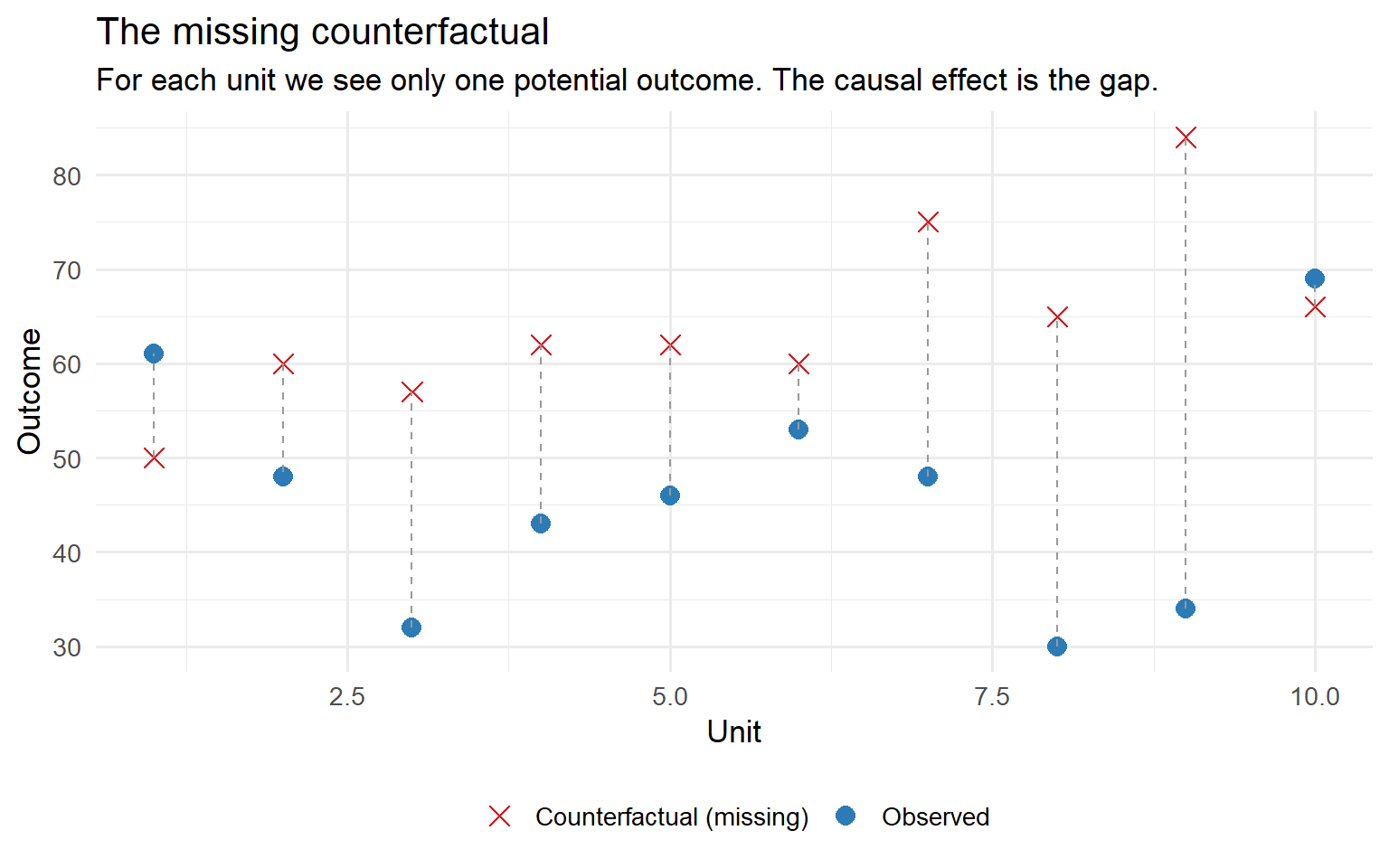
In the real world, each unit of analysis (a customer, a store, a firm, a country) exists in only one state at a time. It either received the treatment, or it did not. We observe one outcome; the other remains permanently hidden.
Holland (1986) formalised this as the Fundamental Problem of Causal Inference. In the potential outcomes framework, due originally to Neyman (1923) and later extended by Rubin (1974), the individual causal effect for unit \(i\) is defined as:
\[\tau_i = Y_i(1) - Y_i(0)\]
where:
- \(Y_i(1)\) is the outcome if unit \(i\) receives treatment,
- \(Y_i(0)\) is the outcome if unit \(i\) does not receive treatment,
- \(\tau_i\) is the individual causal effect.
In practice, we observe \(Y_i(1)\) or \(Y_i(0)\), never both simultaneously. The individual causal effect \(\tau_i\) is, by construction, unidentifiable for a single unit. This is often referred to in the literature as the missing data problem of causal inference (Rubin, 1974; Imbens and Rubin, 2015).
Because we cannot observe both potential outcomes for the same unit, we are forced to construct a plausible counterfactual from other data. The methodology we choose and the assumptions we invoke define the credibility of the entire causal claim.
Prediction versus causal inference
A critical preliminary is the distinction between causal inference and conventional predictive modelling. Conflating the two is the primary source of errors in data-driven strategic decisions.
Prediction asks: given what I observe today, what will happen tomorrow?
Causal inference asks: if I intervene and alter variable \(X\), what happens as a direct consequence of that alteration?
A machine learning model can be outstanding for prediction and entirely uninformative for strategic decision-making. The classical illustration: umbrella sales predict rainfall with high accuracy. Subsidising umbrella production does not cause rain. If you are a public official deciding on drainage infrastructure investment, knowing that “umbrella sales are elevated” is a useful forecast but carries zero causal content.
Pearl (2009) formalised this distinction with the do-calculus. Observational data provides \(P(Y \mid X = x)\), the distribution of outcomes conditional on observing \(X = x\). Causal inference, by contrast, targets \(P(Y \mid do(X = x))\), the distribution of outcomes if we were to force \(X = x\) through an external intervention. These are distinct mathematical objects. The do-operator represents a graph surgery on the causal model: it severs all edges into \(X\) and fixes its value, removing any confounding by variables that previously determined \(X\). Observational conditioning does none of this (Pearl, Glymour, and Jewell, 2016).
This distinction also maps onto Pearl’s three-rung hierarchy of causation (Pearl and Mackenzie, 2018): (1) association, which captures statistical correlations and is sufficient for prediction; (2) intervention, which asks what happens if we act, corresponding to \(do\)-expressions; and (3) counterfactuals, which ask what would have happened to a specific unit under conditions contrary to those actually observed. Standard regression and machine learning operate exclusively at the first rung. Causal inference targets the second and third.
## The identification landscape: how we build counterfactuals
Since the counterfactual is not directly observable, every causal identification strategy is, in practice, an answer to a single question: which other data can validly substitute for the missing potential outcome?
The following table summarises the principal strategies, grouped by the structure of data they exploit, together with their identifying assumptions and key vulnerabilities.
NotePrincipal identification strategies
| Strategy | Core assumption | Counterfactual comes from | Key vulnerability |
|---|---|---|---|
| Randomised experiment (RCT) | Random assignment of treatment | The control group, by construction | External validity (generalisation to real-world conditions) |
| Difference-in-Differences (DiD) | Parallel trends absent treatment | A control group with a parallel time trend | Violation of the parallel trends assumption |
| Synthetic control | A weighted combination of donors fits pre-treatment trends | An artificial composite from a donor pool | Interpolation bias; arbitrary pool selection |
| Regression Discontinuity (RD) | Units just above and below a threshold are comparable | Units on the other side of the cutoff | Strictly local validity (estimates hold only near the cutoff) |
| Instrumental Variables (IV) | Instrument shifts treatment but does not affect the outcome directly | Exogenous variation induced by the instrument | Weak instruments; violation of the exclusion restriction |
| G-computation / G-formula | No unmeasured confounders (conditional exchangeability) | Predicted outcomes from a correctly specified outcome model | Model misspecification |
Each strategy requires a different identifying assumption. The quality of a causal claim is only as strong as the plausibility of that assumption in the specific empirical context.
Building counterfactuals in practice
Consider a common operational scenario: a unit is observed over time, an intervention occurs at a known point, and we want to estimate the intervention’s effect. The counterfactual is the trajectory the unit would have followed in the absence of the intervention.
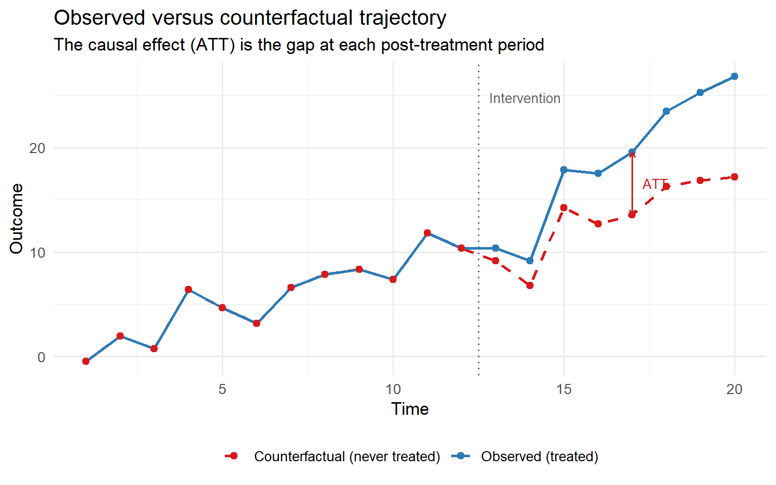
The Average Treatment Effect on the Treated (ATT) is the average gap between the observed and counterfactual trajectories across the post-treatment period. At time \(t\), it is defined as:
\[ATT(t) = E[Y_i(1) - Y_i(0) \mid D_i = 1]\]
The estimation problem is that we observe only one of the two lines. Every identification strategy is a different method for recovering the red dashed line.
Counterfactuals by data structure
The appropriate strategy depends intrinsically on the structure of the available data. The three principal settings are time-series data, panel data, and cross-sectional data with covariates.
Time-series counterfactuals
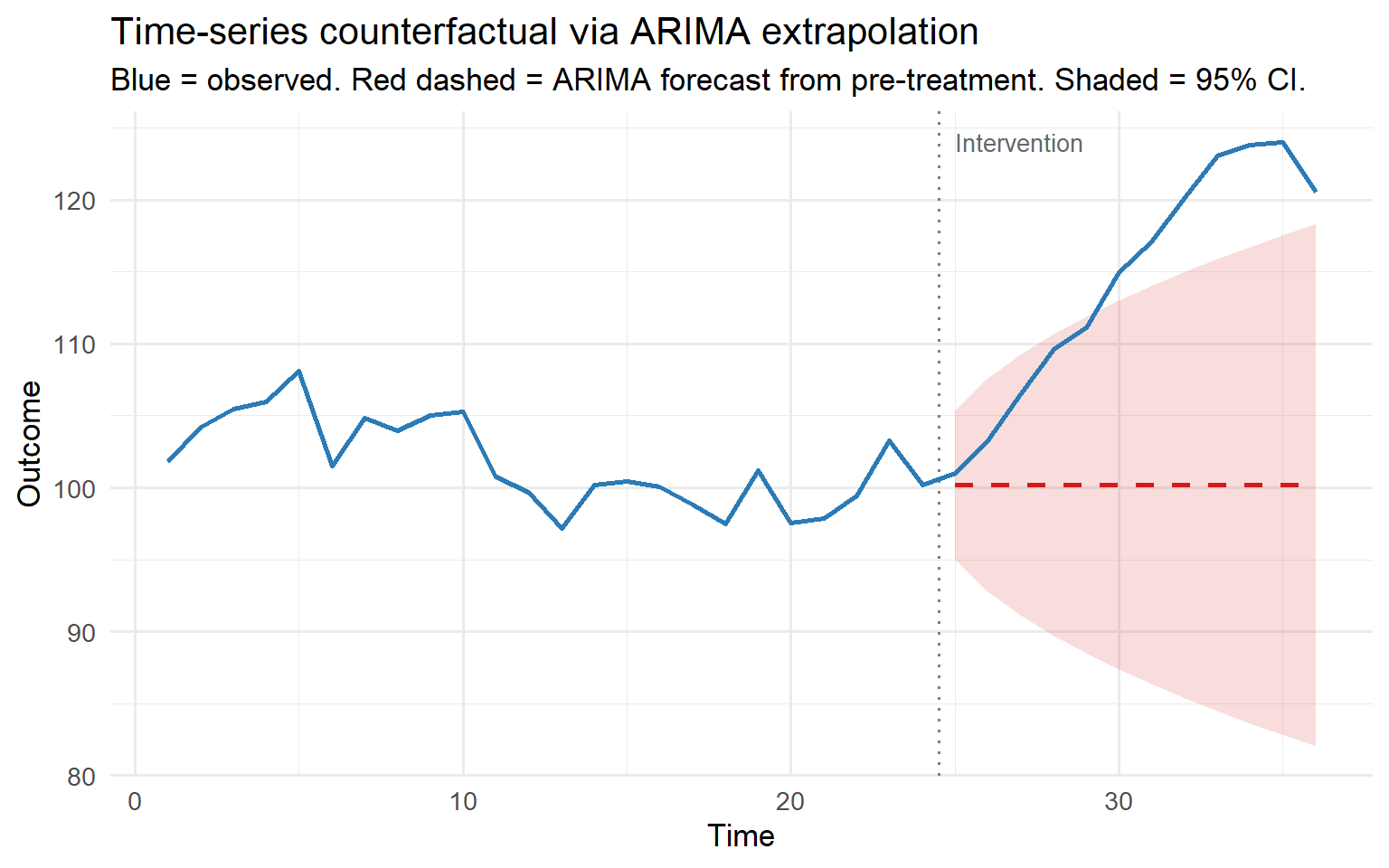
When a single unit is observed over time (a country, a firm, a city) and an intervention occurs at a known date, the counterfactual is the projection of what the series would have done absent the intervention.
The standard tool is to fit a model to the pre-intervention period and extrapolate it into the post-period. This is the logic underlying CausalImpact (Brodersen et al., 2015), which models the pre-treatment period with a Bayesian structural time-series model using auxiliary covariates as controls. It is also the logic of Causal ARIMA (Menchetti, Cipollini, and Mealli, 2023), which extends ARIMA models to a causal inference setting, and of synthetic control methods applied to a single treated unit.
The credibility of this approach depends entirely on two conditions: the quality of the model’s fit during the pre-intervention period, and the absence of other concurrent events (exogenous shocks) that coincide with the intervention. A good in-sample fit does not guarantee a valid out-of-sample extrapolation when there is an unmodelled structural break.
Panel data counterfactuals: Difference-in-Differences
When multiple units are observed over time and only a subset receives treatment, the untreated units can serve as the counterfactual for the treated units. This is the foundation of Difference-in-Differences (DiD).
The key identifying assumption is parallel trends: in the absence of treatment, the treated and control groups would have followed the same temporal trajectory. Under this assumption, the counterfactual for the treated group after treatment is their pre-treatment level plus the trend observed in the control group.
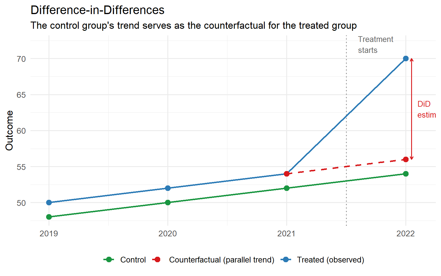
The DiD estimator is:
\[\widehat{ATT} = \underbrace{(\bar{Y}_{\text{treated, post}} - \bar{Y}_{\text{treated, pre}})}_{\text{change in treated}} - \underbrace{(\bar{Y}_{\text{control, post}} - \bar{Y}_{\text{control, pre}})}_{\text{change in control}}\]
The control group’s trend is subtracted from the treated group’s change. The residual, the portion of the change not attributable to a common trend, is the estimated causal effect.
A note on recent methodological developments: the DiD literature has undergone substantial revision since Callaway and Sant’Anna (2021) and Goodman-Bacon (2021) demonstrated that the canonical Two-Way Fixed Effects (TWFE) estimator can produce severely biased estimates under staggered treatment adoption when treatment effects are heterogeneous across cohorts or over time. In such settings, already-treated units can act as “forbidden comparisons” in the TWFE decomposition. Robust alternatives, including the Callaway–Sant’Anna group-time average treatment effect estimator and the stacked regression approach (Baker et al., 2022), are now standard practice for staggered DiD designs.
Cross-sectional counterfactuals: G-computation
When cross-sectional data with covariates are available but no natural control group or time series exists, counterfactuals can still be constructed through G-computation, also known as the g-formula or outcome regression standardisation (Robins, 1986; Hernán and Robins, 2020).
The procedure follows three steps. First, fit an outcome model \(\hat{E}[Y \mid X, D]\) using the observed data. Second, use this fitted model to impute what each unit’s outcome would have been under a hypothetical intervention, that is, setting \(D = 1\) for all units (to obtain \(\hat{Y}_i(1)\)) and setting \(D = 0\) for all units (to obtain \(\hat{Y}_i(0)\)), while holding covariates \(X_i\) fixed at their observed values. Third, compare the two distributions of imputed outcomes.
Under the assumption of conditional exchangeability (also termed no unmeasured confounding or ignorability), which states that treatment assignment is independent of potential outcomes conditional on the observed covariates, \(D \perp\!\!\!\perp \{Y(0), Y(1)\} \mid X\), this procedure yields a consistent estimate of the causal effect (Robins, 1986).
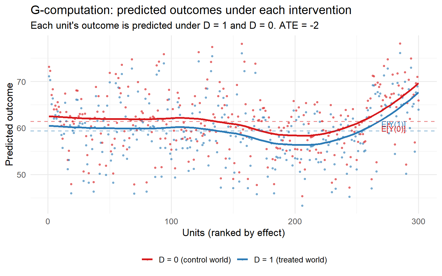
The Average Treatment Effect (ATE) under g-computation is:
\[\widehat{ATE} = \frac{1}{n} \sum_{i=1}^{n} \left[ \hat{E}[Y \mid X_i, D=1] - \hat{E}[Y \mid X_i, D=0] \right]\]
This approach is notably flexible: it accommodates any outcome model, handles both continuous and discrete treatments, and naturally extends to the analysis of heterogeneous treatment effects by examining the distribution of unit-level effects rather than only the mean.
One important distinction concerns the estimand. G-computation as described above targets the ATE, standardising over the full covariate distribution. Restricting the standardisation to the treated units’ covariate distribution yields the ATT; restricting to the untreated units yields the ATU. The practical implication is that the choice of estimand should be determined by the decision question, not by computational convenience (Hernán and Robins, 2020; Arel-Bundock et al., 2024).
The principal vulnerability is model misspecification. If the outcome model is incorrectly specified, the counterfactual predictions inherit that misspecification. This is the rationale for doubly robust estimators such as the Augmented Inverse Probability Weighting (AIPW) estimator (Robins, Rotnitzky, and Zhao, 1994), which combines outcome regression (g-computation) with propensity score weighting. If either model, the outcome model or the propensity score model, is correctly specified, the final estimate remains consistent. Targeted Maximum Likelihood Estimation (TMLE), developed by van der Laan and Rubin (2006), provides a semiparametric, doubly robust alternative that also permits flexible machine learning nuisance models while preserving valid statistical inference.
Three estimands: ATE, ATT, ATU
A recurring source of confusion in applied work is the conflation of distinct causal estimands. G-computation makes the distinction transparent because the estimand is directly determined by the population over which we standardise.
The Average Treatment Effect (ATE) is the expected causal effect if a randomly selected unit from the full population were treated:
\[ATE = E[Y_i(1) - Y_i(0)]\]
The Average Treatment Effect on the Treated (ATT) conditions on the treated subpopulation:
\[ATT = E[Y_i(1) - Y_i(0) \mid D_i = 1]\]
The Average Treatment Effect on the Untreated (ATU) conditions on the control subpopulation:
\[ATU = E[Y_i(1) - Y_i(0) \mid D_i = 0]\]
The ATE, ATT, and ATU coincide when treatment effect heterogeneity is absent or when treatment assignment is independent of potential outcomes (as in a randomised experiment). In observational settings with selection into treatment, the three can differ substantially. A job training programme, for instance, may exhibit a large ATT because the population that self-selects into training differs systematically from those who do not, and the programme may be less effective for the latter group.
Connecting the approaches
The three strategies described above operate on the same underlying logic at different levels of data abstraction:
- What would have happened to this unit had things been different?
- We construct the answer using different sources of variation — time-series trends, cross-unit comparisons, or covariate-adjusted predictions.
- The causal claim is only as credible as the assumption that our constructed counterfactual is a valid stand-in for the unobserved one.
Warning: package 'patchwork' was built under R version 4.4.3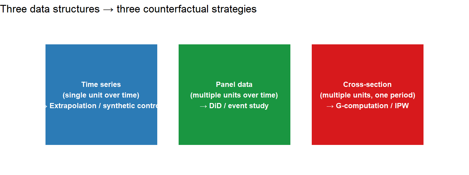
What comes next
This post has introduced the foundational concepts. Subsequent posts will go deeper on each identification strategy:
- Difference-in-Differences: from the canonical 2×2 case to staggered adoption and the pitfalls of TWFE
- Synthetic control: building an artificial counterfactual from a donor pool
- G-computation and doubly robust estimators: when rich covariate data are available but no natural experiment exists
- Regression Discontinuity: exploiting threshold rules for local identification
- Event studies: testing parallel trends and tracing treatment effect dynamics over time
References
- Arel-Bundock, V., Greifer, N., and Heiss, A. (2024). How to Interpret Statistical Models Using marginaleffects for R and Python. Journal of Statistical Software, 111(9), 1–32.
- Baker, A., Callaway, B., Cunningham, S., Goodman-Bacon, A., and Sant’Anna, P.H.C. (2025). Difference-in-Differences Designs: A Practitioner’s Guide. Journal of Economic Literature.
- Brodersen, K.H., Gallusser, F., Koehler, J., Remy, N., and Scott, S.L. (2015). Inferring causal impact using Bayesian structural time-series models. Annals of Applied Statistics, 9(1), 247–274.
- Callaway, B. and Sant’Anna, P.H.C. (2021). Difference-in-Differences with multiple time periods. Journal of Econometrics, 225(2), 200–230.
- Cunningham, S. (2021). Causal Inference: The Mixtape. Yale University Press.
- Goodman-Bacon, A. (2021). Difference-in-differences with variation in treatment timing. Journal of Econometrics, 225(2), 254–277.
- Hernán, M.A. and Robins, J.M. (2020). Causal Inference: What If. Chapman and Hall/CRC.
- Holland, P.W. (1986). Statistics and Causal Inference. Journal of the American Statistical Association, 81(396), 945–960.
- Imbens, G.W. and Rubin, D.B. (2015). Causal Inference for Statistics, Social, and Biomedical Sciences. Cambridge University Press.
- Menchetti, F., Cipollini, F., and Mealli, F. (2023). Combining counterfactual outcomes and ARIMA models for policy evaluation. The Econometrics Journal, 26(1), 1–24.
- Neyman, J. (1923 [1990]). On the application of probability theory to agricultural experiments. Essay on principles. Section 9. Statistical Science, 5(4), 465–480.
- Pearl, J. (2009). Causality: Models, Reasoning, and Inference (2nd ed.). Cambridge University Press.
- Pearl, J., Glymour, M., and Jewell, N.P. (2016). Causal Inference in Statistics: A Primer. Wiley.
- Pearl, J. and Mackenzie, D. (2018). The Book of Why: The New Science of Cause and Effect. Basic Books.
- Robins, J.M. (1986). A new approach to causal inference in mortality studies with a sustained exposure period: application to control of the healthy worker survivor effect. Mathematical Modelling, 7, 1393–1512.
- Robins, J.M., Rotnitzky, A., and Zhao, L.P. (1994). Estimation of regression coefficients when some regressors are not always observed. Journal of the American Statistical Association, 89(427), 846–866.
- Rubin, D.B. (1974). Estimating causal effects of treatments in randomized and nonrandomized studies. Journal of Educational Psychology, 66(5), 688–701.
- van der Laan, M.J. and Rubin, D. (2006). Targeted maximum likelihood learning. International Journal of Biostatistics, 2(1).