---
title: "Propensity Score Done Right: A Masterclass in Observational Causal Inference"
subtitle: "From the regression illusion to sensitivity analysis: a six-step playbook for a €4M decision."
description: "A complete, code-first masterclass on estimating a causal effect from observational data: why OLS is an illusion under poor overlap, how the propensity score restores a data-verified comparison, matching and weighting, machine learning for the propensity score, doubly robust estimation, the sensitivity analysis that stress-tests the whole thing, and a decision matrix that maps business questions to methods. Full R implementation throughout."
date: 2026-07-27
categories: [causal inference, propensity score, machine learning, R]
---
A large European retailer spent €4 million scaling a seller onboarding programme on the strength of a single number: a 23% lift in Gross Merchandise Value, read off the coefficient of one OLS regression. The number was an illusion. Not because the programme did nothing, and not because the estimate was large, but because the regression never estimated the programme's effect in the first place. It estimated the shape of a line drawn through a region of the data where no comparable sellers existed. Most observational studies control for confounders by adding them to a regression. On data that looks like this retailer's, that regression is answering a question nobody asked.
The mechanics of the mistake are worth stating precisely, because they recur in almost every observational business analysis. The team fit `lm(log_gmv_post ~ enrolled + log_gmv_pre + tenure + category + country)`, read a coefficient of 0.21 on `enrolled`, and reported a 23% lift, since $\exp(0.21) - 1 \approx 0.234$. But enrolled sellers were systematically higher-tenure, concentrated in high-performing product categories, and clustered in DACH markets. OLS did not correct for these differences. It extrapolated across regions of covariate space where no comparable untreated sellers existed, and the coefficient it returned reflected the parametric projection of a straight line into empty space, not a data-driven comparison between similar sellers. The standard error around that 0.21 was small, which made the estimate look trustworthy. Precision around a biased number is not evidence. It is a more confident way of being wrong.
This is a masterclass, longer and more complete than the usual post in this series, because getting an observational estimate right is not a single technique but a sequence of decisions, each of which can quietly break the conclusion. It develops a full six-step playbook for the retailer's problem, progressing from the diagnosis of OLS failure to the formal stress-testing of the final estimate against confounders no one measured. A regression coefficient is not a causal effect. It becomes one only when the comparison behind it is supported by data, not by the line a model draws through the gaps. The six steps:
- **The regression illusion.** OLS produces a coefficient, not a causal effect. Non-collapsibility distorts logistic coefficients when prognostic covariates are added or removed, and extrapolation outside common support makes the estimate model-dependent. The propensity score reduces the full covariate vector to a scalar that is sufficient for identification under unconfoundedness.
- **Matching enforces overlap.** Pair each enrolled seller with a comparable non-enrolled seller, discard the incomparable, and verify balance via standardised mean differences below 0.1. Matching is nonparametric preprocessing that makes the outcome model far less sensitive to specification.
- **Weighting keeps the full pool.** Instead of discarding sellers, reweight the control pool to mirror the enrolled. IPW, CBPS, and Entropy Balancing solve the balance problem with different robustness properties, and the effective sample size must be checked before any result is reported.
- **Machine learning escapes the logit trap.** When selection is highly non-linear, logistic regression fails silently for the propensity score. Gradient boosting via `twang` estimates it flexibly, tuned for covariate balance rather than prediction accuracy.
- **Doubly robust estimation is the safety net.** AIPW and Double Machine Learning combine a propensity model with an outcome model and stay consistent if either is right. Cross-fitting and Neyman orthogonality make ML plug-in estimators safe for inference, with one warning: a collider in the outcome model destroys the guarantee.
- **Sensitivity analysis is the non-negotiable stress test.** Every method above assumes no unmeasured confounding. `sensemakr` and E-values quantify how strong an unobserved confounder would need to be to overturn the conclusion. An observational study presented without sensitivity analysis is professionally incomplete.
Full R implementation throughout.
## Executive Summary
A large European retailer invested €4 million in scaling a seller onboarding programme based on a naive OLS estimate of approximately 23% GMV lift (a coefficient of 0.21 on log GMV, implying $\exp(0.21) - 1 \approx 23.4\%$; the commonly cited "21%" conflates a log-point difference with a percentage change). That estimate is almost certainly wrong. Enrolled sellers were systematically higher-tenure, concentrated in high-performing product categories, and clustered in DACH markets. OLS did not correct for these differences; it extrapolated across regions of covariate space where no comparable untreated sellers existed, and the reported coefficient reflected parametric projection rather than data-driven comparison.
This article develops a complete, six-step causal playbook for estimating the programme's effect on Gross Merchandise Value (GMV), progressing from the identification of OLS failure modes to the formal stress-testing of the final estimate against unmeasured confounding.
- **The Regression Illusion.** OLS produces a coefficient, not a causal effect. Non-collapsibility distorts logistic regression coefficients when prognostic covariates are added or removed, and extrapolation outside common support makes the OLS estimate model-dependent. The propensity score solves the dimensionality problem by reducing the full covariate vector to a scalar that is sufficient for identification under unconfoundedness.
- **Matching Enforces Overlap.** Pair each enrolled seller with a similar non-enrolled seller using the propensity score, discard the incomparable ones, and verify balance via Standardised Mean Differences below 0.1. Matching is nonparametric preprocessing that makes subsequent outcome models far less sensitive to specification.
- **Weighting Keeps the Full Seller Pool.** Instead of discarding sellers, reweight the control pool to mirror the enrolled sellers. Inverse Probability Weighting (IPW), Covariate Balancing Propensity Scores (CBPS), and Entropy Balancing each solve the balance problem with different robustness properties. The Effective Sample Size (ESS) must be checked before any result is reported.
- **Machine Learning Escapes the Logit Trap.** When the relationship between seller characteristics and programme selection is highly non-linear (involving threshold effects, interactions, and quadratic terms), logistic regression fails silently for the propensity score. Gradient Boosting Machines via `twang` estimate the propensity score flexibly, tuned for covariate balance rather than prediction accuracy.
- **Doubly Robust Estimation Is the Ultimate Safety Net.** AIPW and Double Machine Learning combine a propensity score model with an outcome model, remaining consistent if either is correctly specified. Cross-fitting and Neyman orthogonality make ML plug-in estimators safe for inference. The critical warning: collider bias in the ML outcome model destroys the double robustness property regardless of the propensity score model.
- **Sensitivity Analysis Is the Non-Negotiable Stress Test.** Every method above assumes no unmeasured confounding. `sensemakr` quantifies how strong an unobserved confounder (such as intrinsic seller motivation) would need to be to overturn the conclusion. E-values translate that vulnerability into a single risk-ratio number that a CFO can evaluate with domain knowledge. An observational study presented without sensitivity analysis is professionally incomplete.
## Part 1. The Problem: The Regression Illusion
A large European retailer is evaluating a seller onboarding programme. Enrolled sellers receive dedicated account management, structured training, and expedited catalogue approval. The question is simple: does the programme lift Gross Merchandise Value (GMV)?
The analytics team has 18 months of seller-level data, 4,200 enrolled sellers and 31,000 controls, with pre-enrolment GMV, seller tenure, category mix, and country. The instinct is immediate: *run OLS and control for everything.*
```r
lm(log_gmv_post ~ enrolled + log_gmv_pre + tenure + category + country,
   data = sellers)
```
The coefficient on `enrolled` comes back at 0.21. The team interprets this as a 21% GMV lift and allocates €4M to scale the programme.
**Log transformation and percentage interpretation.** When the outcome is $\log(\text{GMV})$, a coefficient of $\beta$ corresponds to a multiplicative change of $\exp(\beta) - 1$, not $\beta$. The approximation $\exp(\beta) - 1 \approx \beta$ is accurate only for coefficients below roughly 0.10. For $\beta = 0.21$, it overstates the discrepancy by 2.4 percentage points, small in absolute terms but meaningful for business decisions and for precise academic writing. Throughout this article we work with the log-point coefficient; any conversion to a percentage must use the exponential transformation.
This is almost certainly wrong. Not because the estimate is large, but because the identification strategy is unverified.
### Two Sources of Bias in Observational Estimates
Before examining the failure modes, it is worth framing the problem with a decomposition that Keele & Grieve (2025) make explicit. For any estimator of a causal effect, the total error decomposes into hidden bias, misspecification bias, and statistical noise.
**Hidden bias** arises from unmeasured confounders: variables that affect both treatment assignment and the outcome but are absent from the dataset. This is a design problem; no statistical method can fix it without additional data or assumptions. Sensitivity analysis (Part 6) quantifies how much hidden bias it would take to overturn the result.
**Misspecification bias** arises from incorrect functional-form assumptions in the statistical model. If the true relationship between a covariate and the outcome is quadratic but the model assumes linearity, the treatment effect estimate is biased. If the true propensity score depends on an interaction between tenure and category mix but the logistic regression includes only main effects, the weights will be wrong. This is a modelling problem, and it is the primary motivation for every method in Parts 2 through 5.
**Statistical noise** is the familiar sampling variability that shrinks with sample size and is captured by standard errors and confidence intervals.
The critical insight: **misspecification bias does not shrink with sample size.** A misspecified model estimated on 100,000 sellers is just as biased as one estimated on 1,000; it is merely more precisely wrong. This is why OLS can report a tiny standard error around a badly biased estimate, and why the 21% GMV lift could be both statistically significant and causally meaningless.
Misspecification can operate in two directions. **Under-specification** omits relevant terms (nonlinearities, interactions) from the model, producing bias. **Over-specification** includes irrelevant terms, inflating variance without adding bias. In practice, the threat is almost always under-specification: the true data-generating process contains structure that the analyst's model does not capture. But over-specification matters too: adding hundreds of polynomial and interaction terms to a logistic regression in pursuit of flexibility can produce weights so variable that the effective sample size collapses. The entire trajectory of methods in this article, from matching through doubly robust ML, is about navigating between these two risks.
#### Misspecification Bias Can Rival Omitted Variable Bias
Keele & Grieve (2025) and Goff (2014) make a point that practitioners routinely underestimate: **misspecifying the functional form of a control variable can bias the treatment effect estimate as much as omitting that variable entirely.** The intuition is that an incorrectly specified covariate fails to absorb the confounding it is supposed to block, leaving residual confounding that flows directly into the treatment coefficient.
The simulation below demonstrates this in the retailer's context. The true outcome model contains a quadratic effect of tenure on GMV. We compare three OLS specifications: (1) omitting tenure entirely, (2) including tenure but assuming a linear effect (misspecified), and (3) including the correct quadratic specification.
```{r}
#| label: sim-misspec-vs-omitted
#| warning: false
#| message: false
set.seed(2025)
n <- 5000

# Covariates
tenure   <- rnorm(n)
enrolled <- rbinom(n, 1, plogis(0.5 * tenure))

# True outcome: quadratic tenure effect, true treatment effect = 1.5.
# Because the treatment effect is constant (does not depend on tenure or
# other covariates), ATE = ATT = 1.5 by construction.
log_gmv  <- 1.5 * enrolled + 2 * tenure + 1.5 * tenure^2 + rnorm(n, sd = 2)
true_ATE <- 1.5  # equals ATT here due to constant treatment effect

# Model 1: Omit tenure entirely
fit_omit  <- lm(log_gmv ~ enrolled)
bias_omit <- coef(fit_omit)["enrolled"] - true_ATE

# Model 2: Include tenure as linear (misspecified functional form)
fit_misspec  <- lm(log_gmv ~ enrolled + tenure)
bias_misspec <- coef(fit_misspec)["enrolled"] - true_ATE

# Model 3: Correct specification (quadratic)
fit_correct  <- lm(log_gmv ~ enrolled + tenure + I(tenure^2))
bias_correct <- coef(fit_correct)["enrolled"] - true_ATE

results <- data.frame(
  Specification = c("Omit tenure", "Linear tenure (misspecified)", "Quadratic tenure (correct)"),
  ATE_estimate  = round(c(coef(fit_omit)["enrolled"],
                          coef(fit_misspec)["enrolled"],
                          coef(fit_correct)["enrolled"]), 4),
  Bias          = round(c(bias_omit, bias_misspec, bias_correct), 4)
)
knitr::kable(results,
  caption = paste0("Misspecification bias vs. omitted variable bias. True ATE = ",
                   true_ATE, ". Linear tenure specification produces bias comparable to omitting tenure entirely."))
```
The result is striking: specifying tenure as linear when its true effect is quadratic leaves bias of similar magnitude to omitting tenure altogether. The misspecified model "controls for" tenure in name only; the residual quadratic variation in tenure that the linear term cannot absorb continues to confound the treatment effect. This is why the methods in Parts 2 through 5, which are less reliant on correct functional-form specification, are not academic refinements but practical necessities.
### What OLS Actually Does
The linear model
$$
Y_i = \tau D_i + X_i^{\top}\beta + \varepsilon_i
$$
where $D_i$ is treatment, $X_i$ is the covariate vector, and $Y_i$ is the outcome, identifies the causal effect $\tau$ only under two conditions that are rarely stated and almost never verified:
**1. Correct functional form.** The conditional expectation $E[Y \mid D, X]$ is linear and additive in $X$, with no unmodelled interactions or nonlinearities. In practice this is an assumption about every cross-partial derivative of the response surface.
**2. Common support with no extrapolation.** The regression is fitted over the full joint support of $X$ in the data. When treated and control units occupy different regions of covariate space, OLS silently extends the parametric surface into regions where no counterfactual observations exist.
Conditional exchangeability, $\{Y_i(1), Y_i(0)\} \perp D_i \mid X_i$, is the *identification* condition. But identification and estimation are separate problems. Ho, Imai, King & Stuart (2007) showed that OLS maps that identification condition onto a causal estimate only when both conditions above hold. Outside the region of common support, or under any misspecification of the functional form, what the coefficient measures is the model's own extrapolation, not a causal effect.
For the retailer: enrolled sellers were systematically higher-tenure and higher-GMV, concentrated in two product categories. The OLS fit extrapolates across a region of covariate space where no comparable untreated sellers exist. The 0.21 is model-dependent, not data-driven.
::: {.callout-warning title="Common mistake"}
Interpreting the OLS coefficient on a treatment indicator as causal when treated and control units do not overlap in covariate space. Adding more controls to a misspecified or imbalanced regression compounds the problem; it does not fix it.
:::
### Two Precise Failure Modes of Regression
#### Failure Mode 1: Non-Collapsibility
**Definition: Non-collapsibility.** A treatment effect measure is *non-collapsible* if the marginal effect (averaged unconditionally over the covariate distribution) differs from a weighted average of the conditional effects (at fixed values of $X$), even in the complete absence of confounding. The odds ratio from logistic regression is non-collapsible. The risk difference and the absolute risk reduction from linear probability models are collapsible. The hazard ratio from Cox regression is also non-collapsible.
In linear regression, the coefficient on $D$ does not change when you add a covariate $X$ that is independent of $D$ and predictive of $Y$, because collapsibility holds. In logistic regression this is false. Adding a covariate that predicts $Y$, even one with zero correlation to $D$ (hence not a confounder in any sense), changes the coefficient on $D$. This is not model misspecification; it is a mathematical property of the logistic link function.
The practical consequence: the marginal log-odds ratio (from a model without $X$) and the conditional log-odds ratio (from a model with $X$) are *different estimands*. Switching between them by adding or removing prognostic covariates does not make the estimate "more adjusted"; it changes what is being estimated.
Consider the retailer's context. If an analyst models the probability that a seller's GMV exceeds a threshold using logistic regression, two analysts with identical data who differ only in which prognostic covariates they include will report materially different "treatment effects." Neither is statistically wrong. They are estimating different quantities. The marginal OR does not identify the conditional causal effect; the conditional OR does not identify the population-average effect without further standardisation. Regression output conceals this distinction entirely.
The simulation below makes this concrete. We generate binary $Y$ with a true conditional log-OR for treatment of exactly $1.0$, and a strong prognostic covariate $X$. $D$ and $X$ are independent by construction, so $X$ is not a confounder. The crude model (without $X$) attenuates the coefficient substantially; only the adjusted model recovers the true parameter.
```{r}
#| label: sim-noncollapsibility
#| warning: false
#| message: false
set.seed(2025)
n <- 20000

# D and X are independent: zero confounding by construction
D <- rbinom(n, 1, 0.5)
X <- rnorm(n)

# True conditional log-OR for D is 1.0; X has a strong prognostic effect
# but is NOT a confounder (Cor(D,X) approx 0)
Y <- rbinom(n, 1, plogis(0 + 1.0 * D + 2.0 * X))

m_crude <- glm(Y ~ D,     family = binomial)
m_adj   <- glm(Y ~ D + X, family = binomial)

results <- data.frame(
  Model        = c("Crude: Y ~ D", "Adjusted: Y ~ D + X"),
  `Log-OR (D)` = round(c(coef(m_crude)["D"], coef(m_adj)["D"]), 4),
  `OR (D)`     = round(exp(c(coef(m_crude)["D"], coef(m_adj)["D"])), 3),
  check.names  = FALSE
)
knitr::kable(
  results,
  caption = paste0(
    "Non-collapsibility. Cor(D, X) = ", round(cor(D, X), 4),
    " (X is not a confounder). True conditional log-OR = 1.000. ",
    "The crude model attenuates by ",
    round((1.0 - coef(m_crude)["D"]) / 1.0 * 100, 1),
    "% relative to the true parameter."
  )
)
```
::: {.callout-warning title="Common mistake"}
Interpreting logistic or Cox regression coefficients on $D$ as marginal causal effects. The conditional log-OR from a logistic regression is not the marginal log-OR, and the gap between them widens as the prognostic power of the included covariates increases. To recover a marginal causal effect on the **risk difference** scale from a logistic model, you must standardise over the covariate distribution (g-computation). The marginal log-OR has no standard causal interpretation under the potential-outcomes framework and should not be the estimand of interest in policy evaluations; the marginal risk difference or marginal risk ratio is preferable. This step is almost never taken in practice.
:::
#### Failure Mode 2: Extrapolation Outside Common Support
**Definition: Common support.** The region of common support is the subset of covariate space where both treated and control units exist with positive probability:
$$
\mathcal{S} = \{\, x : 0 < \Pr(D = 1 \mid X = x) < 1 \,\}
$$
Within $\mathcal{S}$, for every covariate profile there is a nonzero chance of observing a unit from each group. Outside $\mathcal{S}$, causal identification requires functional-form assumptions that cannot be tested against the data.
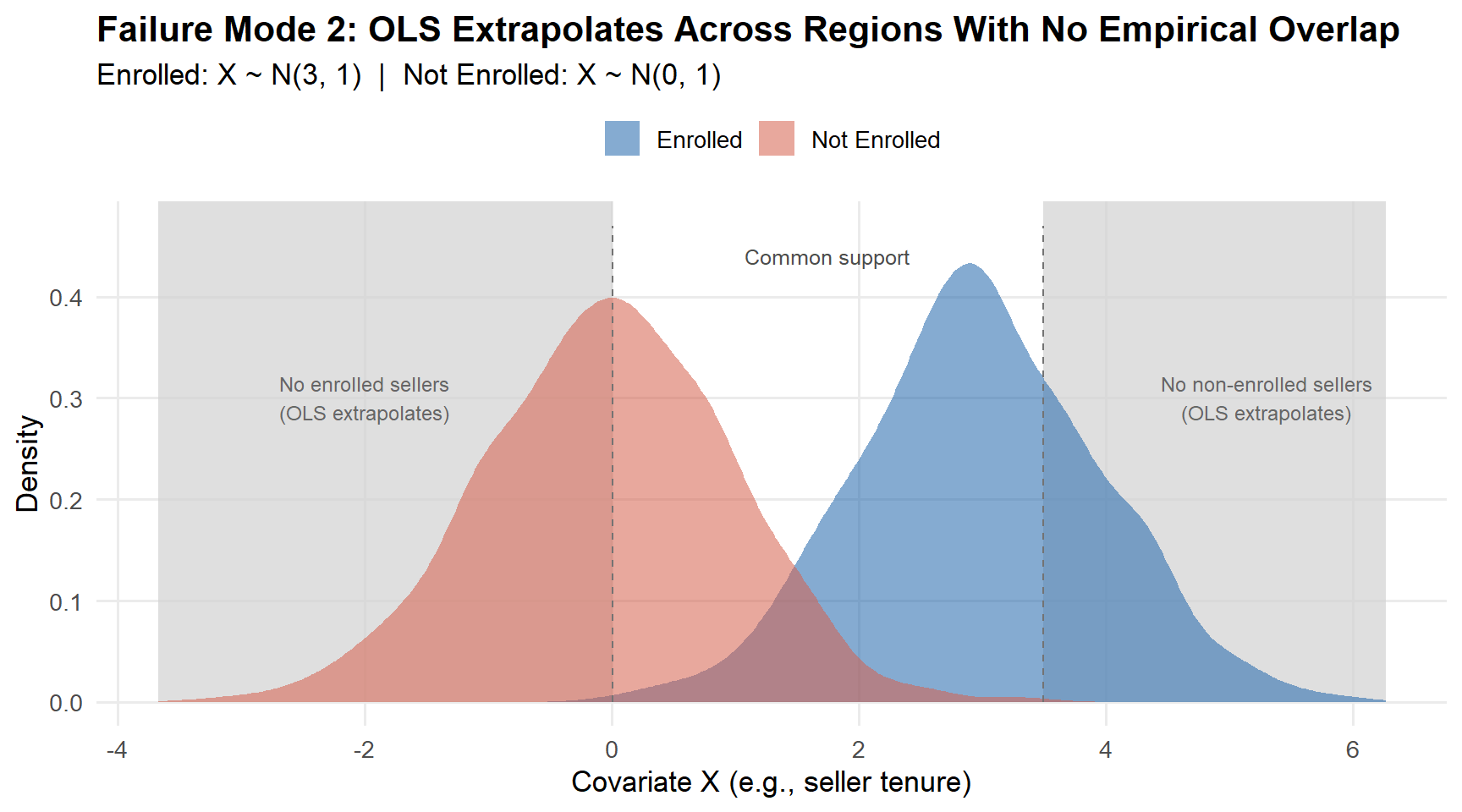
OLS does not stop at the boundary of $\mathcal{S}$. It fits a global surface and extrapolates. When enrolled sellers cluster at high tenure and non-enrolled sellers cluster at low tenure, the model projects its linear slope into the empty space between them, imputing counterfactual outcomes from the parametric assumption rather than from observations. Different functional forms (linear, quadratic, cubic) extrapolate differently, producing arbitrarily different causal estimates from the same data. Ho et al. (2007) demonstrated that in real observational datasets, the variance of treatment effect estimates across reasonable model specifications collapses by an order of magnitude once the non-overlapping units are removed.
The figure below makes the problem visible. Enrolled sellers come from $X \sim N(3, 1)$, non-enrolled sellers from $X \sim N(0, 1)$. The shaded regions contain essentially no units from one group; OLS extrapolates across both.
```{r}
#| label: fig-common-support
#| fig-cap: "Covariate distributions for enrolled (blue) and non-enrolled (orange) sellers. Shaded regions mark where one group is absent; OLS extrapolates here using parametric assumptions alone, not data."
#| warning: false
#| message: false
#| fig-width: 9
#| fig-height: 5
library(ggplot2)
set.seed(42)
n_t <- 500
n_c <- 1000
X_treated <- rnorm(n_t, mean = 3, sd = 1)
X_control <- rnorm(n_c, mean = 0, sd = 1)

dat <- data.frame(
  X     = c(X_treated, X_control),
  Group = factor(
    rep(c("Enrolled", "Not Enrolled"), c(n_t, n_c)),
    levels = c("Enrolled", "Not Enrolled")
  )
)

overlap_lo <- max(min(X_treated), min(X_control))
overlap_hi <- min(max(X_treated), max(X_control))

ggplot(dat, aes(x = X, fill = Group)) +
  annotate("rect",
    xmin = min(X_control) - 0.3, xmax = overlap_lo,
    ymin = 0, ymax = Inf, fill = "grey82", alpha = 0.7
  ) +
  annotate("rect",
    xmin = overlap_hi, xmax = max(X_treated) + 0.3,
    ymin = 0, ymax = Inf, fill = "grey82", alpha = 0.7
  ) +
  geom_density(alpha = 0.55, colour = NA) +
  scale_fill_manual(values = c("Enrolled" = "#2166AC", "Not Enrolled" = "#D6604D")) +
  annotate("segment",
    x = overlap_lo, xend = overlap_lo, y = 0, yend = 0.47,
    linetype = "dashed", colour = "grey45", linewidth = 0.5
  ) +
  annotate("segment",
    x = overlap_hi, xend = overlap_hi, y = 0, yend = 0.47,
    linetype = "dashed", colour = "grey45", linewidth = 0.5
  ) +
  annotate("text",
    x = (overlap_lo + overlap_hi) / 2, y = 0.44,
    label = "Common support", size = 3.3, colour = "grey30"
  ) +
  annotate("text",
    x = -2.0, y = 0.30,
    label = "No enrolled sellers\n(OLS extrapolates)",
    hjust = 0.5, size = 3.1, colour = "grey40"
  ) +
  annotate("text",
    x = 5.3, y = 0.30,
    label = "No non-enrolled sellers\n(OLS extrapolates)",
    hjust = 0.5, size = 3.1, colour = "grey40"
  ) +
  labs(
    title    = "Failure Mode 2: OLS Extrapolates Across Regions With No Empirical Overlap",
    subtitle = "Enrolled: X ~ N(3, 1)  |  Not Enrolled: X ~ N(0, 1)",
    x        = "Covariate X (e.g., seller tenure)",
    y        = "Density",
    fill     = NULL
  ) +
  theme_minimal(base_size = 13) +
  theme(
    legend.position  = "top",
    plot.title       = element_text(face = "bold"),
    panel.grid.minor = element_blank()
  )
```
The result is *model dependence* (Ho et al., 2007; Rosenbaum & Rubin, 1983): small changes in functional form, such as adding $X^2$ or including an interaction, can swing the point estimate arbitrarily because different models extrapolate differently into the empty covariate regions. The reported standard error captures none of this uncertainty. It conditions on the model being correct.
::: {.callout-tip title="Practical rule"}
Plot the covariate distributions for enrolled and non-enrolled sellers before fitting any outcome model. If the distributions are visually separated, you have an overlap problem that no regression specification can fix. The correct responses are: (i) restrict inference to the region of common support, (ii) redefine the estimand to the overlap population, or (iii) collect more data.
:::
### The Propensity Score: Dimensionality Reduction for Identification
Both failure modes share a root: OLS conditions on the high-dimensional vector $X$ through a parametric model, leaving the distribution of $X$ unexamined and the region of extrapolation invisible. The propensity score works in covariate space first, making comparability a data-verified property rather than a modelling assumption.
**Definition: Propensity score (Rosenbaum & Rubin, 1983).** For a unit with pre-treatment covariates $X_i$, the propensity score is
$$
e(X_i) = \Pr(D_i = 1 \mid X_i).
$$
It is the conditional probability of receiving treatment given the full covariate vector.
#### The Balancing Property
**Theorem (Rosenbaum & Rubin, 1983, Theorem 1).** Conditional on the propensity score, the covariate vector $X$ is independent of treatment assignment:
$$
D_i \perp X_i \mid e(X_i).
$$
The intuition: two sellers with the same $e(X)$ had the same probability of being enrolled, regardless of their individual covariate values. Conditional on $e(X)$, knowing $X$ adds no information about who received treatment; the assignment looks locally random within propensity score strata.
#### The Sufficiency Result
The balancing property directly yields the key identification corollary.
**Corollary (Rosenbaum & Rubin, 1983, Theorem 3).** If conditional exchangeability holds given $X$,
$$
\{Y_i(1), Y_i(0)\} \perp D_i \mid X_i,
$$
then it also holds given the scalar $e(X_i)$ alone:
$$
\{Y_i(1), Y_i(0)\} \perp D_i \mid e(X_i).
$$
The intuition is direct: if $X$ was sufficient to block all confounding paths between $D$ and the potential outcomes, and $e(X)$ is sufficient to balance $X$ across treatment groups, then $e(X)$ alone is sufficient for identification. One scalar replaces the full covariate vector.
#### Why This Solves the Dimensionality Problem
With $p$ covariates, conditioning nonparametrically on $X$ requires data in a $p$-dimensional space; the data requirement grows exponentially in $p$ (the curse of dimensionality). With $p$ binary covariates, there are $2^p$ possible strata, most of which will be empty.
The propensity score collapses this to a single scalar. Instead of requiring enrolled and non-enrolled sellers to match on all $p$ dimensions simultaneously, you only need units to have similar values of $e(X)$. One number per seller replaces $p$ numbers, and the balancing property guarantees this scalar is sufficient for identification.
#### The Diagnostic That Regression Never Gives You
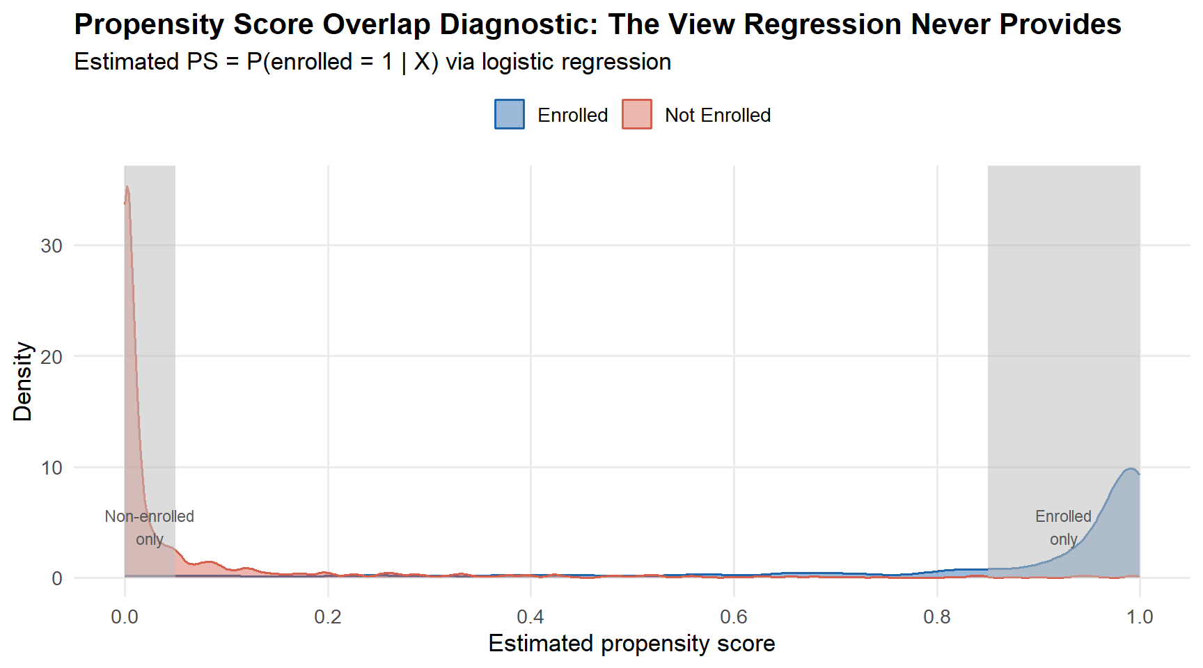
The propensity score makes overlap *visible*. Estimate $e(X)$, plot its distribution separately for enrolled and non-enrolled sellers, and you see immediately where comparable units exist and where they do not. This is the single most important pre-analysis diagnostic in observational causal inference, and it is completely absent from standard regression output.
```{r}
#| label: fig-ps-density
#| fig-cap: "Propensity score distributions for enrolled (blue) and non-enrolled (orange) sellers, estimated via logistic regression on the same data as the previous figure. Mass concentrated near 0 or 1 signals a common support violation, visible here before any outcome model is fitted."
#| warning: false
#| message: false
#| fig-width: 9
#| fig-height: 5
# Reuse the same data as the common support figure above
dat_ps <- data.frame(
  X = c(X_treated, X_control),
  D = c(rep(1L, n_t), rep(0L, n_c))
)

# Estimate propensity score via logistic regression
ps_model     <- glm(D ~ X, data = dat_ps, family = binomial)
dat_ps$ps    <- predict(ps_model, type = "response")
dat_ps$Group <- factor(
  ifelse(dat_ps$D == 1, "Enrolled", "Not Enrolled"),
  levels = c("Enrolled", "Not Enrolled")
)

ggplot(dat_ps, aes(x = ps, fill = Group, colour = Group)) +
  geom_density(alpha = 0.45, linewidth = 0.7) +
  annotate("rect",
    xmin = 0, xmax = 0.05, ymin = 0, ymax = Inf,
    fill = "grey75", alpha = 0.55
  ) +
  annotate("rect",
    xmin = 0.85, xmax = 1.0, ymin = 0, ymax = Inf,
    fill = "grey75", alpha = 0.55
  ) +
  scale_fill_manual(values   = c("Enrolled" = "#2166AC", "Not Enrolled" = "#D6604D")) +
  scale_colour_manual(values = c("Enrolled" = "#2166AC", "Not Enrolled" = "#D6604D")) +
  annotate("text", x = 0.025, y = 4.6,
    label = "Non-enrolled\nonly",
    hjust = 0.5, size = 3.0, colour = "grey35"
  ) +
  annotate("text", x = 0.925, y = 4.6,
    label = "Enrolled\nonly",
    hjust = 0.5, size = 3.0, colour = "grey35"
  ) +
  scale_x_continuous(limits = c(0, 1), breaks = seq(0, 1, 0.2)) +
  labs(
    title    = "Propensity Score Overlap Diagnostic: The View Regression Never Provides",
    subtitle = "Estimated PS = P(enrolled = 1 | X) via logistic regression",
    x        = "Estimated propensity score",
    y        = "Density",
    fill     = NULL,
    colour   = NULL
  ) +
  theme_minimal(base_size = 13) +
  theme(
    legend.position  = "top",
    plot.title       = element_text(face = "bold"),
    panel.grid.minor = element_blank()
  )
```
The figure is unambiguous. Non-enrolled sellers concentrate near $e(X) = 0$; enrolled sellers concentrate near $e(X) = 1$. Overlap is minimal. Any causal estimate built on this data without first addressing the overlap failure is an extrapolation, and the propensity score plot makes that visible before a single outcome is modelled.
Compare this to the standard regression workflow: OLS produces a point estimate and a standard error. Nothing in that output indicates whether the comparison is supported by data or by parametric projection into empty covariate space.
::: {.callout-tip title="Diagnostic rule"}
Always plot propensity score distributions for enrolled and non-enrolled sellers before any outcome analysis. If the densities are severely separated, no estimator is valid without restricting the sample to the region of common support. This applies equally to matching, weighting, and regression.
:::
## Part 2. Matching: Enforcing Overlap
Knowing $e(X)$ is necessary but not sufficient. The propensity score tells you who is comparable to whom, but does not by itself produce a valid causal estimate. The estimation step requires a deliberate choice of how to use $e(X)$: match on it, weight by its inverse, or combine both in a doubly robust estimator.
Matching is the first and most transparent approach. For the retailer, matching means finding, for each enrolled seller, a non-enrolled seller with a similar propensity score, and discarding the "weird" sellers (both enrolled and non-enrolled) who have no counterpart in the other group.
### What Matching Does (and Does Not Do)
Matching is **nonparametric preprocessing**, not an estimator. Following Ho et al. (2007), it is a design-based procedure that restructures the observed data prior to any outcome analysis. It prunes the sample to a region of common support and reweights or re-selects control units so that the empirical distribution of pre-treatment covariates is similar between treatment groups. Any subsequent outcome model then operates over units that are genuinely comparable, making estimates far less sensitive to functional-form assumptions and free from extrapolation outside the region of common support.
Matching as implemented in `MatchIt` is a form of **subset selection**: the pruning and weighting of units to arrive at a (weighted) subset of the units from the original dataset. When done successfully, subset selection produces a new sample where treatment is unassociated with the covariates, so that a comparison of outcomes between groups is not confounded by the measured and balanced covariates.
Matching is nonparametric in the sense that the estimated weights and pruning of the sample are not direct functions of estimated model parameters but rather depend on the organisation of discrete units in the sample; this contrasts with propensity score weighting, where the weights come more directly from the estimated propensity score model and are therefore more sensitive to its correct specification.
It is important to note that this implementation of matching differs from the methods described by Abadie and Imbens (2006, 2016) and implemented in the `Matching` R package and the `teffects` routine in Stata. That form of matching is **matching imputation**, where the missing potential outcomes for each unit are imputed using the observed outcomes of paired units. This is a critical distinction because matching imputation is a specific estimation method with its own effect and standard error estimators, in contrast to subset selection, which is a preprocessing method that does not require specific estimators and is broadly compatible with other analyses.
The default estimand for most matching procedures is the **Average Treatment Effect on the Treated (ATT)**:
$$
\tau_{\text{ATT}} = E[\, Y_i(1) - Y_i(0) \mid D_i = 1 \,].
$$
This is the natural quantity in the retailer's evaluation: *what was the effect of the programme on sellers who actually participated?* Standard matching algorithms retain every treated unit and search for comparable controls, so the matched sample inherently represents the treated population. If the estimand of interest is the population ATE rather than the ATT, different tools are needed: full matching with `estimand = "ATE"`, subclassification, or propensity score weighting.
### Formal Definition of Balance
A matched sample satisfies **balance** when the empirical distribution of covariates is approximately equal across treatment groups:
$$
\tilde{p}(X \mid D = 1) \approx \tilde{p}(X \mid D = 0),
$$
where $\tilde{p}$ denotes the **empirical** distribution in the matched sample. Balance is a **sample property**, not a population hypothesis. It is assessed by comparing distributional summaries in the matched data, not by hypothesis testing against a super-population.
### Matching Is Not an Estimator
After matching you still need to estimate the treatment effect. The common practice of reporting a simple difference in means on the matched sample is valid only after **exact matching** (where within-pair covariate differences are identically zero). In virtually every other case, residual within-pair imbalance remains, and a simple difference in means ignores it, producing a biased point estimate. Moreover, a simple difference in means treats matched pairs as independent observations, producing standard errors that ignore the matched structure and are therefore anti-conservative. The correct approach is a **weighted regression on the matched sample** incorporating the matching weights produced by `matchit()`, with **cluster-robust standard errors clustered on** `subclass` (pair membership) (Greifer & Stuart, 2021; Ho et al., 2007).
### The Matching Pipeline in Practice
A rigorous matching analysis follows four sequential steps. Critically, Steps 1 through 3 constitute the **design phase** and must be completed **without consulting the outcome variable**. The outcome is examined only after a matching specification has been finalised, protecting the analysis from confirmation bias (Ho et al., 2007).
#### Step 1: Estimate the Propensity Score
The propensity score $e(X)$ is typically estimated by logistic regression of the treatment indicator on the pre-treatment covariates:
$$
e(X_i) = \frac{1}{1 + \exp(-X_i^{\top}\beta)}.
$$
This is a **prediction problem, not a causal model**. The coefficients $\beta$ carry no structural interpretation; they parameterise the conditional probability of treatment assignment. Their sole purpose is to produce a ranking of units that, when used for matching, yields good covariate balance. The correct specification of the propensity score model is judged exclusively by whether matching on it achieves balance, not by the model's AUC, pseudo-$R^2$, or the significance of individual coefficients (Austin, 2009; Ho et al., 2007).
If post-matching balance diagnostics reveal residual imbalance on any covariate, return to this step: add interactions, polynomial terms, or splines, then rematch and re-check balance. Let the balance diagnostics guide specification; never the outcome data.
::: {.callout-warning title="Never use the propensity score as a covariate in the outcome regression"}
Including $e(X)$ as a predictor in the outcome model is **not** propensity score adjustment; it is ordinary regression with an extra variable. It provides no balancing guarantee, does not enforce common support, and does not reduce model dependence. The propensity score is a matching or weighting tool, not a control variable (Ho et al., 2007).
:::
#### Step 2: Choose a Matching Algorithm
`MatchIt` (Ho et al., 2011) implements a wide range of matching methods. At the heart of `MatchIt` are three classes of methods: **distance matching**, **stratum matching**, and **pure subset selection**. Distance matching involves selecting control units to pair with each treated unit based on the distance between units; stratum matching creates strata based on unique values of the covariates; pure subset selection selects subsets to optimise a criterion subject to balance and sample size constraints.
##### Nearest-Neighbour Matching (1:1, Without Replacement)
For each treated unit $i$, find the control unit $j$ minimising the absolute propensity score distance:
$$
j^{*}(i) = \arg\min_{j \in \mathcal{C}(i)} \; \bigl| \hat{e}(X_i) - \hat{e}(X_j) \bigr|,
$$
where $\mathcal{C}(i)$ is the pool of as-yet-unmatched control units. The algorithm is **greedy**: it processes treated units sequentially (by default in descending order of the propensity score, so the hardest-to-match units are paired first) and commits to each match without revising earlier decisions. Because matched controls are removed from the pool, each control is used at most once. Nearest-neighbour matching is the most common form of matching used (Thoemmes & Kim, 2011) and is implemented in `MatchIt` using internal C++ code through `Rcpp`, making it extremely fast even for large datasets.
##### Optimal Pair Matching
Optimal pair matching (`method = "optimal"`) attempts to choose matches that collectively minimise the sum of the absolute pair distances in the matched sample (Hansen & Klopfer, 2006; Gu & Rosenbaum, 1993), rather than greedily. Optimal pair matching in `MatchIt` depends on the `fullmatch()` function in the `optmatch` package. Optimal pair matching and nearest-neighbour matching often yield the same or very similar matched samples (Austin, 2013), but optimal matching requires computing the full distance matrix between units, which may make it inapplicable to very large datasets.
##### k:1 Matching and Matching with Replacement
**k:1 matching** pairs each treated unit with $k$ controls. Increasing $k$ preserves precision by preventing too many control units from being unmatched, though the gain diminishes rapidly after $k = 4$ (Rosenbaum, 2020). Austin (2010b) found that 1:1 or 1:2 matching generally performed best in terms of mean squared error. **Matching with replacement** allows the same control unit to serve as a match for multiple treated units, reducing bias but inflating variance.
##### Full Matching
Full matching (`method = "full"`) assigns **every unit** to a subclass, each containing at least one treated and at least one control unit. No units are discarded (except those outside common support), making full matching more statistically efficient. It is optimal in the sense of minimising a weighted average of within-subclass distances (Hansen, 2004; Stuart & Green, 2008). Full matching also supports targeting the ATE (set `estimand = "ATE"`), which nearest-neighbour matching cannot do naturally.
##### Genetic Matching
Genetic matching (`method = "genetic"`) uses a genetic algorithm to find scaling factors for each variable in a generalised Mahalanobis distance formula (Diamond & Sekhon, 2013), directly optimising covariate balance rather than relying on the propensity score alone.
##### Coarsened Exact Matching (CEM)
CEM (`method = "cem"`) coarsens each covariate into substantively meaningful bins, performs exact matching on the coarsened data, and retains the original uncoarsened values for analysis (Iacus, King, & Porro, 2012). It belongs to the *Monotonic Imbalance Bounding* (MIB) class of methods. Because exact and coarsened exact matching aim to balance the entire joint distribution of covariates, they are the most powerful methods when feasible.
##### Subclassification
Subclassification (`method = "subclass"`) creates strata based on coarsened versions of the propensity score. When no units are discarded, either the ATT, ATC, or ATE can be estimated, making it one of the few methods that naturally supports the ATE estimand.
##### Cardinality and Profile Matching
Cardinality and profile matching (`method = "cardinality"`) are methods of pure subset selection that guarantee a minimum level of balance by selecting the largest subset satisfying balance constraints (Cohn & Zubizarreta, 2022).
#### Customising the Matching Specification
Beyond the choice of matching method, `MatchIt` provides several options for customising the specification. These options can be combined with any compatible matching method and often make the difference between adequate and excellent balance.
##### Caliper Matching (`caliper`)
A **caliper** limits how far apart matched units can be on a specified variable. Any units for which there are no available matches within the caliper are dropped from the matched sample.
::: {.callout-important title="Always use a caliper"}
Without a caliper, the greedy algorithm will match every enrolled seller to *some* non-enrolled seller, even when they are far apart in covariate space. Impose a caliper of $0.2$ standard deviations on the logit scale (Austin, 2011). In `matchit()`, set `caliper = 0.2` and `std.caliper = TRUE`. Enrolled sellers with no eligible match within the caliper are dropped, narrowing the estimand from the full-population ATT to the **matched-sample ATT**; report this explicitly.
:::
##### Mahalanobis Distance Matching (`mahvars`)
To perform Mahalanobis distance matching within a propensity score caliper, set the `distance` argument to the PS estimation method, specify the `caliper` argument, and supply variables to `mahvars`. This combination is one of the most effective matching specifications (Rubin, 1980).
##### Exact Matching as an Argument (`exact`)
Combining exact matching on a few key nominal variables (e.g., country group) with propensity score matching on the remaining covariates is a powerful and frequently recommended strategy.
##### Common Support Restrictions (`discard`)
The `discard` argument controls whether and how units outside the region of common support are treated before matching begins. This is a separate mechanism from caliper-based trimming.
#### Choosing a Matching Method
Choose based on the dataset's characteristics and the analysis goals. The criteria are **balance** and **remaining (effective) sample size** after matching.
##### Decision Guide for Choosing a Matching Method
| Goal | Recommended Method(s) |
|:---|:---|
| ATT, simple and fast | Nearest neighbour with caliper |
| ATT, optimise pair quality | Optimal pair matching |
| ATT, best balance | Genetic matching; profile matching |
| ATT, retain all treated | Full matching; generalised full matching |
| ATE | Full matching; subclassification; profile matching |
| Guarantee balance bounds | Cardinality matching; profile matching |
| Few covariates, all discrete | Exact matching |
| Mix of discrete + continuous | CEM; or exact on discrete + nearest on continuous |
| Large datasets | Nearest neighbour; generalised full matching |
#### Step 3: Assess Balance
Balance is the **only** criterion that matters when evaluating a matching specification. Not the propensity score model's goodness of fit, not the AUC, not the $p$-value of the treatment coefficient.
##### Primary Diagnostic: Standardised Mean Difference
For each covariate $k$, compute
$$
\text{SMD}_k = \frac{\bar{X}_{k,T} - \bar{X}_{k,C}}{s_{k}},
$$
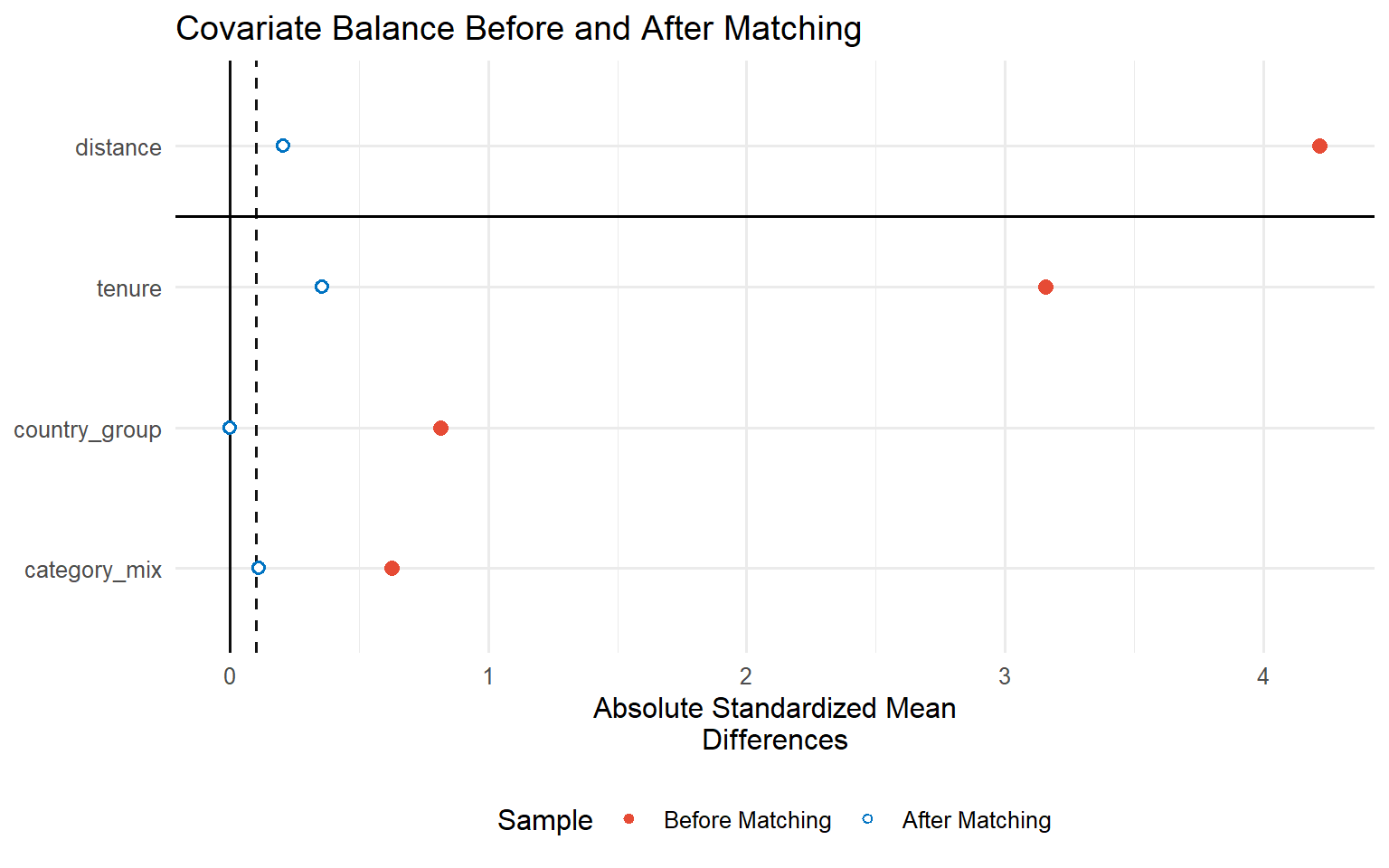
where $\bar{X}_{k,T}$ and $\bar{X}_{k,C}$ are the covariate means in the treated and control groups of the matched sample, and $s_{k}$ is the **pooled standard deviation computed in the original unmatched sample**. The accepted threshold for adequate balance is $|\text{SMD}_k| < 0.1$ for all covariates (Austin, 2009).
##### Secondary Diagnostics
**Variance ratios** should be close to 1 in the matched sample. Values outside $[0.5, 2]$ indicate residual distributional imbalance. **eCDF statistics** detect imbalances in tails and distributional shape. The **Love plot** is the standard reporting vehicle, produced by `cobalt::love.plot()`.
::: {.callout-warning title="Do not use hypothesis tests to assess balance"}
$t$-tests, Wilcoxon tests, and Kolmogorov-Smirnov tests conflate sample size with balance. In a large sample, trivially small covariate differences will be statistically significant; in a small sample, large imbalances may fail to reach significance. Use the SMD, variance ratios, and eCDF statistics instead (Ho et al., 2007; Imai, King, & Stuart, 2008).
:::
##### Simulation: Matching Enrolled Sellers and Assessing Balance
The following code generates a moderately imbalanced observational dataset of sellers, performs 1:1 nearest-neighbour matching with a 0.2 SD caliper on the logit scale, and produces a balance summary and Love plot.
```{r}
#| label: fig-love-matching
#| fig-cap: "Love plot: absolute SMDs before (red) and after (blue) 1:1 nearest-neighbour matching with a 0.2 SD caliper. All post-matching SMDs fall below the 0.1 threshold (Austin, 2009)."
#| warning: false
#| message: false
library(MatchIt)
library(cobalt)
library(ggplot2)
library(sandwich)
library(lmtest)

set.seed(42)
n_enrolled <- 400
n_control  <- 600

sellers <- data.frame(
  enrolled      = c(rep(1, n_enrolled), rep(0, n_control)),
  tenure        = c(rnorm(n_enrolled, mean = 3, sd = 1),   rnorm(n_control, mean = 0, sd = 1)),
  category_mix  = c(rnorm(n_enrolled, mean = 1, sd = 1.5), rnorm(n_control, mean = 0, sd = 1.5)),
  country_group = c(rbinom(n_enrolled, 1, 0.70),           rbinom(n_control, 1, 0.30))
)

# 1:1 NN matching; caliper = 0.2 x SD(logit(PS)): Austin (2011)
m_out <- matchit(
  enrolled ~ tenure + category_mix + country_group,
  data        = sellers,
  method      = "nearest",
  distance    = "glm",
  link        = "logit",
  caliper     = 0.2,
  std.caliper = TRUE,
  replace     = FALSE
)

# Numerical balance summary
summary(m_out, standardize = TRUE)
# Love plot via cobalt
love.plot(
  m_out,
  stats        = "mean.diffs",
  threshold    = 0.1,
  abs          = TRUE,
  binary       = "std",
  colors       = c("#E64B35", "#0073C2"),
  shapes       = c("circle", "circle filled"),
  sample.names = c("Before Matching", "After Matching"),
  var.order    = "unadjusted",
  title        = "Covariate Balance Before and After Matching",
  xlab         = "|Standardised Mean Difference|"
) +
  theme_minimal(base_size = 12) +
  theme(legend.position = "bottom")
```
#### Step 4: Estimate the Treatment Effect on the Matched Sample
With balance confirmed, estimate the ATT using the matched data and the weights produced by `matchit()`. The recommended approach is a **weighted regression of log GMV on the enrolment indicator** and (optionally) the covariates, with the matching weights supplied via the `weights` argument:
$$
\log \text{GMV}_i = \alpha + \tau D_i + X_i^{\top}\beta + \varepsilon_i.
$$
The coefficient $\tau$ estimates the ATT. Including covariates after matching has already balanced them is the "double adjustment" principle (Ho et al., 2007; Rubin & Thomas, 2000): matching handles large, non-linear imbalances and enforces common support, while including $X$ in the outcome regression absorbs any residual imbalance within matched pairs, reduces the variance of the effect estimate, and makes the final estimate doubly robust.
::: {.callout-important title="Always use the matching weights in the outcome model"}
For 1:1 nearest-neighbour matching without replacement, all matched units receive a weight of 1 and unmatched units receive 0, so the weights appear redundant. However, for k:1 matching, full matching, or matching with replacement, units carry variable weights that are essential for correct estimation. Always pass `weights = weights` (or use `match_data()`) to your outcome model. For standard errors, cluster-robust SEs clustered on `subclass` (pair membership) are recommended after pair matching (Greifer & Stuart, 2021).
:::
```{r}
#| label: sim-matched-att
#| warning: false
#| message: false
set.seed(2024)
n <- 1000
tenure       <- rnorm(n)
category_mix <- rnorm(n)

# True DGP: ATT = 2.0 by construction
ps_true  <- plogis(-0.5 + 1.2 * tenure + 0.8 * category_mix)
enrolled <- rbinom(n, 1, ps_true)
log_gmv  <- 2.0 * enrolled + 1.5 * tenure - 0.8 * category_mix + rnorm(n, sd = 1.5)

sim_sellers <- data.frame(log_gmv = log_gmv, enrolled = enrolled,
                          tenure = tenure, category_mix = category_mix)

# Naive OLS on raw data (no matching, no covariate adjustment)
ols_naive      <- lm(log_gmv ~ enrolled, data = sim_sellers)
naive_estimate <- coef(ols_naive)[["enrolled"]]
naive_se       <- sqrt(vcov(ols_naive)["enrolled", "enrolled"])

# 1:1 NN matching with caliper
m_sim <- matchit(
  enrolled ~ tenure + category_mix,
  data        = sim_sellers,
  method      = "nearest",
  distance    = "glm",
  caliper     = 0.2,
  std.caliper = TRUE,
  replace     = FALSE
)
md <- match.data(m_sim)

# Weighted regression with double adjustment on matched data
fit_matched <- lm(log_gmv ~ enrolled + tenure + category_mix,
                  data = md, weights = weights)

# Cluster-robust SEs clustered on matched pairs
vcov_cl     <- vcovCL(fit_matched, cluster = ~subclass, type = "HC1")
matched_est <- coef(fit_matched)[["enrolled"]]
matched_se  <- sqrt(vcov_cl["enrolled", "enrolled"])

results <- data.frame(
  Estimator      = c("Naive OLS (raw, no covariates)",
                     "Matched + weighted OLS (double adjustment)"),
  Estimate       = round(c(naive_estimate, matched_est), 3),
  SE             = round(c(naive_se, matched_se), 3),
  Bias_from_true = round(c(naive_estimate - 2.0, matched_est - 2.0), 3)
)
print(results)
```
The naive OLS estimate is biased because enrolment is correlated with `tenure` and `category_mix`, which also affect GMV. Matching breaks this link by ensuring each enrolled seller is paired with a non-enrolled seller of similar propensity, and the subsequent covariate-adjusted regression absorbs residual imbalance within pairs. The matched estimate recovers the true ATT of 2.0 with substantially less bias.
### When Matching Fails
#### Poor Overlap
When propensity score distributions of enrolled and non-enrolled sellers barely overlap, caliper matching discards a large fraction of enrolled sellers. The estimand silently shifts from the population ATT to a **local matched-sample ATT**. This is defensible (Crump et al., 2009) but must be flagged explicitly. Report the proportion of enrolled sellers successfully matched. If fewer than roughly 80% find acceptable matches, consider weighting methods or redefine the target population.
#### High-Dimensional Covariates
With many covariates, caliper matching in propensity score space does not guarantee individual covariate balance: two sellers can be close on the estimated propensity score while differing substantially on a specific prognostically important covariate. **CEM** and **genetic matching** are robust alternatives. For very high-dimensional settings, **Mahalanobis distance matching within a propensity score caliper** (using the `mahvars` argument) combines the strengths of both approaches.
#### Residual Imbalance After Matching
If any covariate has $|\text{SMD}| > 0.1$ after matching, the specification is inadequate. The iterative remedy is: re-specify the propensity score model with interactions or splines; try a more flexible matching algorithm; add exact matching constraints on the most problematic covariates; and if balance remains elusive, switch to weighting or doubly robust estimation.
::: {.callout-tip title="Optimise for balance, not for model fit"}
Try multiple propensity score specifications and multiple matching algorithms. Choose the specification that produces the best balance across all covariates, **without looking at the outcome data**. This separation of design and analysis is the bedrock of matching's credibility as an observational study design (Ho et al., 2007).
:::
Matching enforces overlap and improves balance, but it does so by discarding data. When the control reservoir is small, the estimand is the ATE rather than the ATT, or overlap is poor, discarding unmatched sellers is wasteful and changes the estimand in ways that are difficult to communicate to decision-makers. Weighting retains every seller and assigns each a weight designed to balance the covariate distributions.
## Part 3. Weighting: Keeping the Full Seller Pool
Matching discards sellers to enforce balance. Weighting does the same job without discarding anyone. Instead of pruning to a balanced subset, weighting assigns each seller a scalar weight to construct a **pseudo-population** in which treatment assignment is independent of covariates. Every seller stays in the analysis, or at least that is where you start. A seller with a low propensity score in the treatment group is rare and informative; it receives a large weight. A seller near $e(X) = 0.5$ is unremarkable; it receives a modest weight. The result is a reweighted sample where the covariate distributions are identical across treatment arms, and a weighted difference in means recovers the causal effect under the same unconfoundedness assumption established in Part 1.
### Formal Weight Definitions
Let $D_i$ be the treatment indicator and $e(X_i)$ the propensity score.
**ATT weights** (the average treatment effect *on the treated*). Enrolled sellers retain weight 1; non-enrolled sellers are reweighted to mirror the enrolled sellers' covariate distribution:
$$
w_i =
\begin{cases}
1 & \text{if } D_i = 1 \\[6pt]
\dfrac{e(X_i)}{1 - e(X_i)} & \text{if } D_i = 0
\end{cases}
$$
**ATE weights** (the average treatment effect in the *full population*). Both arms are reweighted to the marginal distribution of $X$:
$$
w_i =
\begin{cases}
\dfrac{1}{e(X_i)} & \text{if } D_i = 1 \\[8pt]
\dfrac{1}{1 - e(X_i)} & \text{if } D_i = 0
\end{cases}
$$
These are the Horvitz-Thompson weights. The ATT weights set the enrolled group as the reference population. The ATE weights set the overall marginal distribution of $X$ as the reference.
**Weighting is preprocessing, not estimation.** Computing weights is Step 1. Step 2 is estimating the treatment effect using a *weighted* outcome model. The weights create the pseudo-population; the outcome model extracts the effect from it. The estimand matters for every deliverable. An ATT weight targets the effect for sellers actually enrolled. An ATE weight targets the effect if the entire population were enrolled. These are different numbers. Delivering the wrong one is how a correct analysis produces a wrong recommendation.
### The Weighting Pipeline in Practice
#### Step 1: Choose a Weighting Scheme
Three schemes dominate applied work. They differ in what they optimise, how they use the propensity score, and how much robustness they buy against model misspecification.
##### Inverse Probability Weighting (IPW)
The baseline. Estimate $e(X)$ via logistic regression, extract fitted values $\hat{e}(X_i)$, and plug them into the ATT or ATE formulas above. Under a correctly specified propensity score model, IPW achieves the semiparametric efficiency bound for the ATE (Hirano, Imbens & Ridder, 2003).
**Trade-off.** IPW is highly sensitive to propensity scores near 0 or 1. Under ATE estimation, a treated unit with $\hat{e}(X_i) = 0.01$ receives weight $100$. One extreme observation commands the influence of a hundred typical units. Variance explodes. IPW is the right starting point. It is not always the right ending point.
##### Covariate Balancing Propensity Score (CBPS)
Imai & Ratkovic (2014) identified the structural tension in standard IPW: the propensity score is estimated by maximising the likelihood of treatment assignment, not by minimising covariate imbalance. A well-fitted logistic model can still produce weights that leave substantial imbalance in finite samples. CBPS resolves this by estimating the propensity score parameters via the Generalised Method of Moments (GMM), imposing moment conditions that directly require weighted covariate means to be equal across treatment arms. For the ATT, the core moment condition is (Imai & Ratkovic, 2014, eq. 9):
$$
\frac{1}{N} \sum_{i=1}^{N}
\left[ D_i \tilde{X}_i \;-\;
\frac{\hat{e}(X_i)(1 - D_i)}{1 - \hat{e}(X_i)}\,\tilde{X}_i \right] = 0.
$$
**Trade-off.** CBPS improves finite-sample covariate balance relative to standard IPW by directly optimising moment conditions. Under fundamental misspecification of the parametric logistic form, CBPS reduces residual imbalance but shares the same asymptotic bias as standard IPW; it cannot recover the true propensity score if the parametric model is structurally wrong. It still uses a parametric logistic model. If the true assignment mechanism involves interactions or nonlinearities not in your formula, CBPS improves things but cannot fully fix them.
##### Entropy Balancing (EB)
Hainmueller (2012) took the logic of CBPS to its conclusion: if the goal is balance, bypass the propensity score model entirely for the weighting step. Entropy balancing directly solves for weights $w_i$ (for control units) that satisfy prespecified moment conditions while minimising the Kullback-Leibler divergence from uniform base weights:
$$
\min_{w_i} \sum_{i:\, D_i=0} w_i \log\!\left(\frac{w_i}{q_i}\right)
\quad \text{subject to} \quad
\sum_{i:\, D_i=0} w_i \, c_{ri}(X_i) = m_r
\quad \forall\, r \in \{1, \ldots, R\},
$$
where $c_{ri}$ are moment functions and $m_r$ are the corresponding moments of the enrolled group. The result: **exact balance on specified moments by construction**, in every finite sample.
**Trade-off.** EB guarantees balance only on moments you specify. If confounding operates through a higher-order interaction you did not include, EB will not fix it.
#### Step 2: Assess Balance and Weight Diagnostics
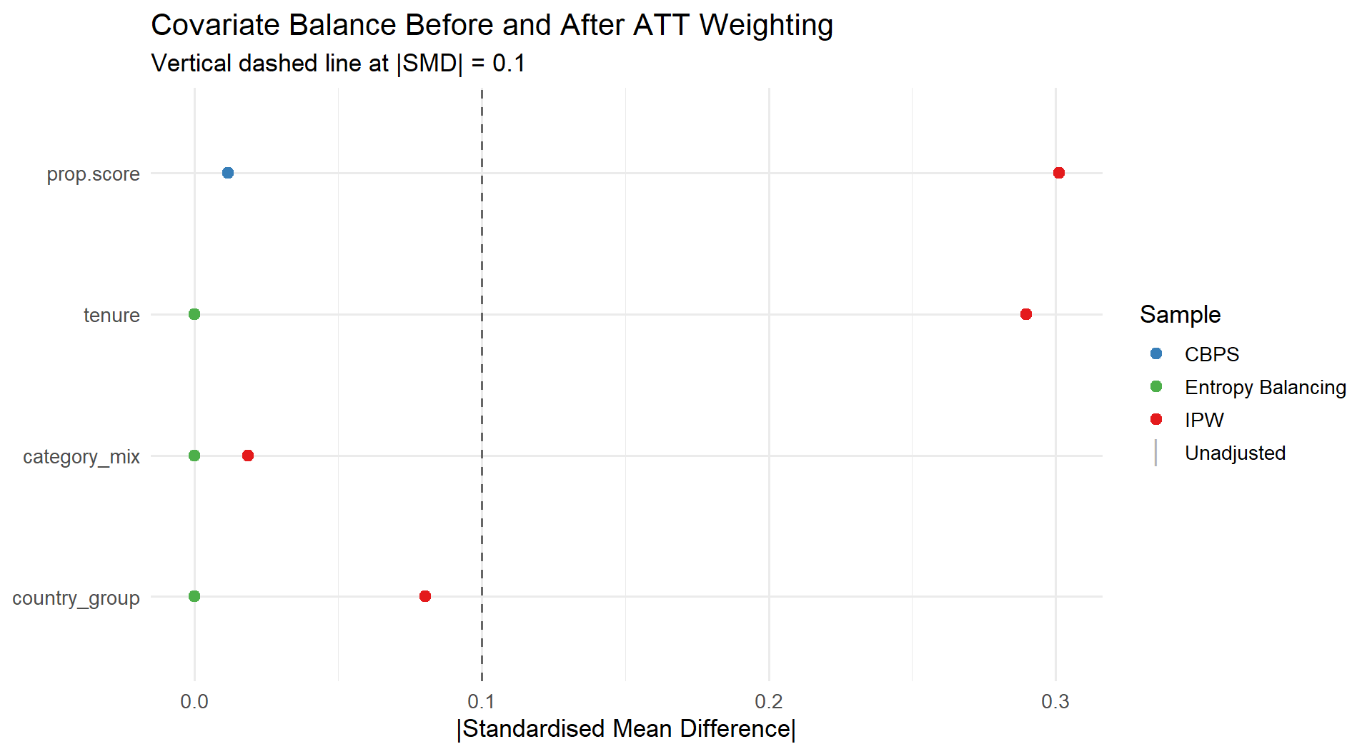
Balance is the only empirical evidence that your identification strategy is working. The primary metric is the **Standardised Mean Difference (SMD)** in the weighted sample, with the threshold $|\text{SMD}| < 0.1$ (Austin, 2009). Do not use $p$-values from balance tests.
**Check the weight distribution, not just the balance statistics.** A Love plot that shows perfect SMDs is meaningless if three observations carry 80% of the analytical weight. Compute the **Effective Sample Size (ESS)**:
$$
\text{ESS} = \frac{\left(\sum_i w_i\right)^2}{\sum_i w_i^2}.
$$
If ESS falls below roughly 30-40% of your nominal sample size, your weights are too extreme. Act on it before reporting results.
#### Step 3: Estimate the Treatment Effect
After establishing balance and verifying the ESS, estimate the treatment effect via weighted regression. Standard errors must account for the weights; the `survey` package implements the Horvitz-Thompson sandwich variance estimator appropriate for probability-weighted designs.
##### Full Simulation: IPW vs. CBPS vs. Entropy Balancing
```{r}
#| label: sim-weighting-data
#| warning: false
#| message: false
library(WeightIt)
library(cobalt)
library(survey)
library(dplyr)

set.seed(20250625)
n <- 2000

# Generate severely imbalanced seller data.
# Treatment assignment is a nonlinear function of covariates:
# includes tenure^2 so a main-effects logit is misspecified,
# and a tenure x country_group interaction to separate CBPS from EB.
tenure        <- rnorm(n)
category_mix  <- rnorm(n)
country_group <- rbinom(n, 1, 0.5)

true_ps <- plogis(-1.2 + 1.5 * tenure + 0.8 * category_mix +
                    0.4 * country_group + 0.5 * tenure^2 +
                    0.3 * tenure * category_mix + 0.4 * tenure * country_group)
enrolled <- rbinom(n, 1, true_ps)
cat("Enrolment prevalence:", round(mean(enrolled), 3), "\n")
# True potential outcomes: true ATT = 2 (constant treatment effect)
true_ATT <- 2
Y0 <- 1.5 * tenure + 0.8 * category_mix + 1.2 * country_group +
      0.4 * tenure^2 + 0.5 * tenure * category_mix + rnorm(n, 0, 1.5)
Y1 <- Y0 + true_ATT
log_gmv <- ifelse(enrolled == 1, Y1, Y0)

dat <- data.frame(log_gmv = log_gmv, enrolled = enrolled,
                  tenure = tenure, category_mix = category_mix,
                  country_group = country_group)
cat("True ATT:", true_ATT, "\n")
```
```{r}
#| label: estimate-weights
#| warning: false
#| message: false
# IPW via logistic regression
w_ipw <- weightit(
  enrolled ~ tenure + category_mix + country_group,
  data     = dat,
  method   = "glm",
  estimand = "ATT"
)

# CBPS: GMM estimation enforcing covariate balance (Imai & Ratkovic, 2014)
w_cbps <- weightit(
  enrolled ~ tenure + category_mix + country_group,
  data     = dat,
  method   = "cbps",
  estimand = "ATT"
)

# Entropy Balancing: bypasses PS, directly optimises weights (Hainmueller, 2012)
w_eb <- weightit(
  enrolled ~ tenure + category_mix + country_group,
  data     = dat,
  method   = "ebal",
  estimand = "ATT"
)

# ESS diagnostics
ess_fn <- function(w) round((sum(w)^2) / sum(w^2), 1)
ctrl   <- dat$enrolled == 0
cat("=== Effective Sample Sizes (control group) ===\n")
cat(" Nominal n_ctrl :", sum(ctrl), "\n")
cat(" IPW ESS :", ess_fn(w_ipw$weights[ctrl]), "\n")
cat(" CBPS ESS :", ess_fn(w_cbps$weights[ctrl]), "\n")
cat(" EB ESS :", ess_fn(w_eb$weights[ctrl]), "\n")
```
```{r}
#| label: fig-love-weighting
#| fig-cap: "Love plot: absolute standardised mean differences before and after ATT weighting for IPW, CBPS, and Entropy Balancing. Vertical dashed line at |SMD| = 0.1."
#| warning: false
#| message: false
#| fig-width: 10
#| fig-height: 5.5
# Compute balance for each weighting method individually (so bal.tab
# dispatches to bal.tab.weightit and resolves the treatment variable from
# the stored weightit metadata), then combine into a single plot.
bt_ipw  <- bal.tab(w_ipw,  stats = "mean.diffs", binary = "std")
bt_cbps <- bal.tab(w_cbps, stats = "mean.diffs", binary = "std")
bt_eb   <- bal.tab(w_eb,   stats = "mean.diffs", binary = "std")

make_smd_df <- function(bt, method) {
  bal <- bt$Balance
  data.frame(
    var    = rownames(bal),
    Unadj  = abs(bal$Diff.Un),
    Adj    = abs(bal$Diff.Adj),
    Method = method,
    stringsAsFactors = FALSE
  )
}

plot_df <- rbind(
  make_smd_df(bt_ipw,  "IPW"),
  make_smd_df(bt_cbps, "CBPS"),
  make_smd_df(bt_eb,   "Entropy Balancing")
)

var_order <- unique(plot_df$var)[order(
  sapply(unique(plot_df$var), function(v) max(plot_df$Unadj[plot_df$var == v])),
  decreasing = TRUE
)]
plot_df$var <- factor(plot_df$var, levels = rev(var_order))

ggplot(plot_df) +
  geom_point(aes(y = var, x = Unadj, colour = "Unadjusted"),
             shape = 124, size = 5, alpha = 0.6) +
  geom_point(aes(y = var, x = Adj, colour = Method), size = 2.5) +
  geom_vline(xintercept = 0.1, linetype = "dashed", colour = "grey40") +
  scale_colour_manual(
    values = c(Unadjusted = "grey50",
               IPW = "#E41A1C", CBPS = "#377EB8",
               `Entropy Balancing` = "#4DAF4A"),
    name = "Sample"
  ) +
  labs(
    title    = "Covariate Balance Before and After ATT Weighting",
    subtitle = "Vertical dashed line at |SMD| = 0.1",
    x        = "|Standardised Mean Difference|",
    y        = NULL
  ) +
  theme_minimal(base_size = 13) +
  theme(legend.position = "right")
```
```{r}
#| label: tbl-weighting-estimates
#| warning: false
#| message: false
# Estimate ATT via weighted regression with robust survey SEs
estimate_att <- function(w_obj, label, data) {
  design <- svydesign(ids = ~1, weights = ~w_obj$weights, data = data)
  fit    <- svyglm(log_gmv ~ enrolled, design = design)
  est    <- coef(fit)["enrolled"]
  se     <- sqrt(diag(vcov(fit)))["enrolled"]
  data.frame(
    Method   = label,
    Estimate = round(est, 3),
    SE       = round(se, 3),
    CI_low   = round(est - 1.96 * se, 3),
    CI_high  = round(est + 1.96 * se, 3),
    row.names = NULL
  )
}

# Naive OLS
ols_fit <- lm(log_gmv ~ enrolled, data = dat)
ols_est <- coef(ols_fit)["enrolled"]
ols_se  <- sqrt(diag(vcov(ols_fit)))["enrolled"]

results <- bind_rows(
  data.frame(
    Method   = "Naive OLS (no adjustment)",
    Estimate = round(ols_est, 3),
    SE       = round(ols_se, 3),
    CI_low   = round(ols_est - 1.96 * ols_se, 3),
    CI_high  = round(ols_est + 1.96 * ols_se, 3),
    row.names = NULL
  ),
  estimate_att(w_ipw,  "IPW (survey SE)",               dat),
  estimate_att(w_cbps, "CBPS (survey SE)",              dat),
  estimate_att(w_eb,   "Entropy Balancing (survey SE)", dat),
  data.frame(
    Method   = "True ATT",
    Estimate = true_ATT,
    SE       = NA_real_,
    CI_low   = NA_real_,
    CI_high  = NA_real_,
    row.names = NULL
  )
)
knitr::kable(results, caption = "ATT estimates: naive OLS vs. three weighted estimators. True ATT = 2.", digits = 3)
```
### The Overlap Problem: Trimming and Stabilization
When $\hat{e}(X)$ approaches 0 or 1, weights explode. These are not numerical inconveniences; they are symptoms of a violated positivity assumption.
#### Trimming Units
Crump et al. (2009) derived the principled response. The practical rule-of-thumb: **discard all sellers with $\hat{e}(X) < 0.1$ or $\hat{e}(X) > 0.9$**, which captures nearly all the variance reduction of the theoretically optimal cut-off.
::: {.callout-warning title="Trimming changes your estimand"}
When you discard sellers with extreme propensity scores, you are no longer estimating the ATT for the original enrolled population. You are estimating the ATT for the **overlapping subpopulation**. Make the estimand shift explicit in every deliverable.
:::
#### Stabilizing Weights
**Stabilized weights** replace the raw ATE numerator of 1 with the marginal treatment probability:
$$
w_i^{\text{stab}} =
\frac{\Pr(D_i = 1)}{\hat{e}(X_i)} \cdot D_i
\;+\;
\frac{\Pr(D_i = 0)}{1 - \hat{e}(X_i)} \cdot (1 - D_i).
$$
Stabilized weights have mean 1 in large samples and reduce variance relative to raw IPW. An alternative is **Overlap Weights**, which concentrate inference on sellers with the most uncertainty about enrolment and naturally bound the weight distribution. These weights target a distinct estimand: the **Average Treatment effect for the Overlap population (ATO)**.
### The ATO Estimand and Overlap Weights (Li, Morgan & Zaslavsky, 2018)
The overlap weight for unit $i$ is $1 - e(X_i)$ for treated units and $e(X_i)$ for control units. These weights are bounded in $[0, 1]$ by construction, eliminating the extreme-weight problem entirely. The corresponding estimand is the **Average Treatment effect for the Overlap population (ATO)**:
$$
\tau_{\text{ATO}} = \frac{E\!\left[\, e(X)\,(1 - e(X))\, \tau(X) \,\right]}{E\!\left[\, e(X)\,(1 - e(X)) \,\right]},
$$
where $\tau(X)$ is the conditional average treatment effect. The overlap weight $e(X)(1 - e(X))$ is maximised at $e(X) = 0.5$ and shrinks toward zero as the propensity score approaches 0 or 1, concentrating inference on the subpopulation where treatment assignment is most uncertain. Unlike the ATT (which targets enrolled sellers) or the ATE (which targets the full seller population), the ATO targets sellers near the decision boundary between enrolment and non-enrolment. The business framing is direct: the ATO answers the question about the sellers with the highest uncertainty of enrolment, the marginal sellers who are most relevant for the decision to scale the programme. When overlap is poor, the ATO is often the only estimand that can be reliably estimated. Available in `WeightIt` via `estimand = "ATO"`.
### When Weighting Fails and What To Do
**Extreme Weights and Positivity Violations.** Solutions, in order of preference: (1) trim using Crump et al. (2009) and restate the estimand; (2) switch to Overlap Weights (`estimand = "ATO"`); (3) if overlap is so severe that trimming drops most enrolled sellers, accept that the data cannot support a credible causal estimate.
**CBPS or EB Fail to Converge.** The failure is informative: no reweighting scheme can manufacture counterfactuals from a region of covariate space where none exist. Options: reduce dimensionality; use regularised PS estimation (`method = "super"` in `WeightIt`); move to doubly robust estimation.
**Residual Imbalance After CBPS and EB.** The true assignment mechanism is genuinely nonlinear in ways your formula does not capture. The solution is to estimate $e(X)$ with a machine learning method that detects and models those nonlinearities automatically.
::: {.callout-tip title="Start simple, escalate only when needed"}
Begin with IPW. Check balance; if all SMDs are below 0.1 and ESS is healthy, stop. If balance fails, move to CBPS. If CBPS leaves imbalance, try EB. If weights are extreme (ESS $<$ 30-40% of $n$), trim or switch to Overlap Weights. Only after all these options are exhausted should you escalate to ML-based PS estimation. Complexity is a cost, not a credential. The best analysis is the simplest one that achieves balance with an acceptable weight distribution.
:::
Every method in this section relies on a parametric model for the propensity score, or assumes the specified moments are sufficient to capture the confounding structure. What if the true relationship between seller characteristics and programme selection is a complex, high-dimensional interaction surface that no logistic regression will capture? If the propensity score model is fundamentally misspecified, the weights are lies. Enter machine learning.
## Part 4. Machine Learning for the Propensity Score
Every weighting estimator from Part 3 (IPW, CBPS, Entropy Balancing) inherits the bias of the propensity score model underneath it. If that model is wrong, the entire causal estimate is wrong. No amount of weighting sophistication rescues a misspecified propensity score.
Standard weighting methods assume a correctly specified model for $e(X)$. In practice, analysts almost always estimate this with logistic regression: main effects, perhaps a few hand-selected interactions, and the implicit assumption that the programme selection mechanism respects a linear additive structure on the log-odds scale. When the true mechanism involves $X^2$, or $X_1 \times X_2$, or a threshold rule, the logistic model is misspecified. The weights are wrong. The bias does not shrink with sample size; it compounds.
::: {.callout-important title="The bottom line"}
A misspecified propensity score model leads to residual confounding and biased treatment effect estimates, regardless of how sophisticated your downstream weighting estimator is. Westreich, Lessler & Funk (2010) demonstrated empirically that misspecified parametric PS models produce materially biased effect estimates in real observational data. This is an operational risk, not a theoretical footnote.
:::
### The ML Pipeline for Propensity Scores
Machine learning offers an escape from the logit trap. The goal is not to use ML to predict outcomes; it is to use ML to estimate the propensity score itself, flexibly and adaptively, without committing to a restrictive parametric form. The pipeline has three steps. Skipping any one of them produces worse results than sticking with logistic regression.
#### Step 1: Choose the ML Algorithm (Beyond Logit)
The workhorse for PS estimation is **Gradient Boosting Machines (GBM)**, implemented in R via the `twang` package. McCaffrey, Ridgeway & Morral (2004) introduced GBM for PS estimation and showed that it consistently outperforms logistic regression in achieving covariate balance when the true treatment assignment mechanism involves complex relationships among many covariates.
GBM builds an ensemble of shallow regression trees sequentially. Each new tree fits the residuals of the previous ensemble. The result is a highly flexible function approximator that automatically captures non-linearities and high-order interactions without manual variable selection or polynomial expansion. You supply the covariates; GBM determines which ones matter and how they combine.
::: {.callout-warning title="ML estimates the PS, not the outcome"}
In causal inference here, we use ML *strictly* to estimate the propensity score. We do **not** use ML to predict the outcome in this step. The outcome model is a separate component. Using ML for both simultaneously without proper cross-fitting introduces overfitting bias into the treatment effect estimate.
:::
#### Step 2: Tuning for Balance, Not Accuracy
This is the most consequential conceptual shift in the entire pipeline. In standard machine learning, you tune hyperparameters to minimise prediction error. In propensity score estimation, **prediction accuracy is the wrong objective**.
A model that predicts programme enrolment with 95% AUC is often overfitting to idiosyncratic patterns in the data, producing propensity scores near 0 and 1. Those scores produce extreme inverse-probability weights. Extreme weights blow up variance and destroy the effective sample size. A model with moderate prediction accuracy but excellent covariate balance produces far better causal estimates.
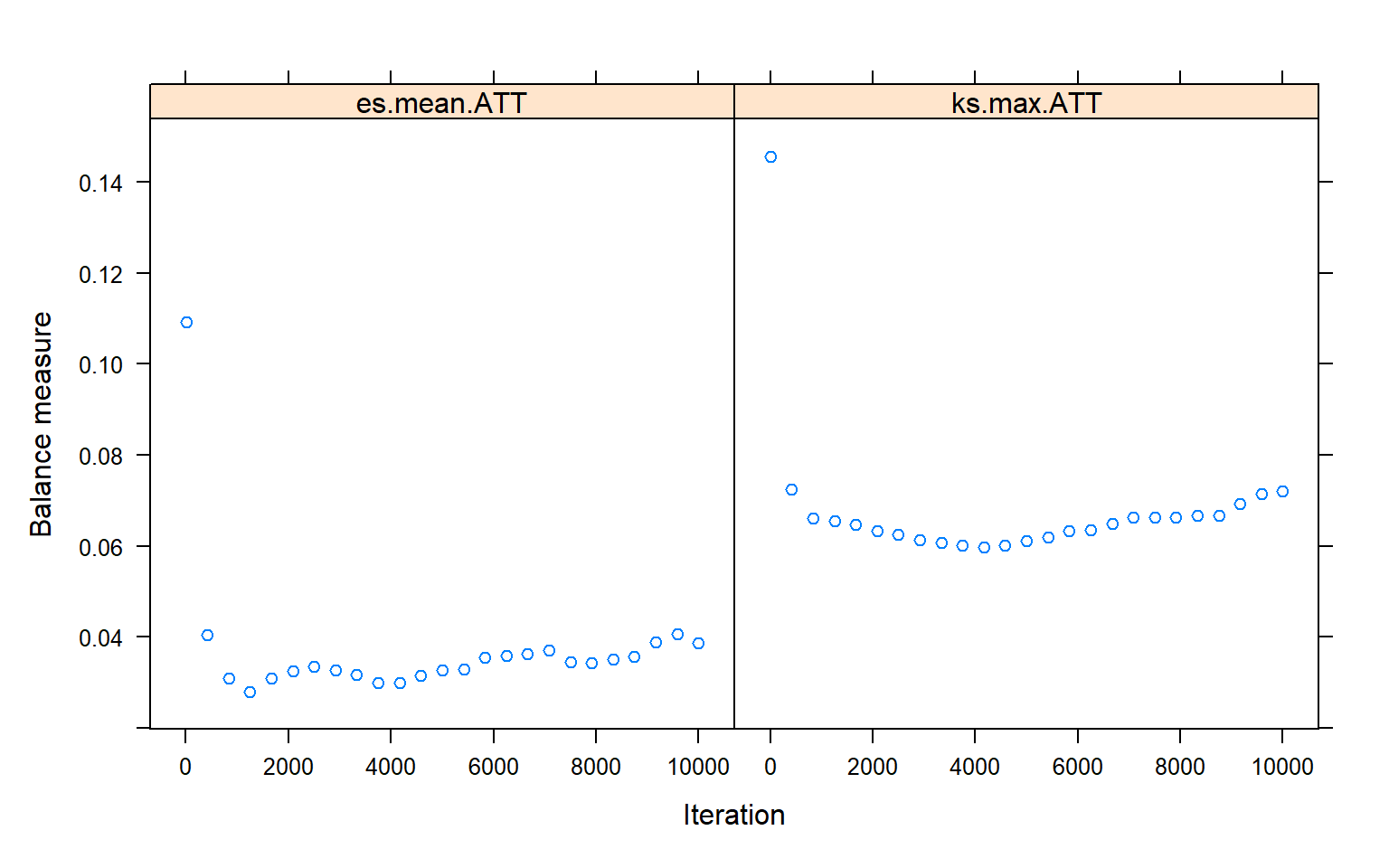
The correct tuning objective is **covariate balance**. The `twang` package implements this directly. The algorithm adds GBM trees iteratively and evaluates balance at each iteration. It stops at the iteration that minimises a chosen balance statistic:
- **`es.mean` / `es.max`**: mean or maximum standardised effect size across all covariates.
- **`ks.mean` / `ks.max`**: mean or maximum Kolmogorov-Smirnov statistic.
The distinction between `.mean` and `.max` matters. Minimising the mean improves average balance but can leave individual covariates badly imbalanced. Minimising the max targets the worst-balanced covariate directly. Use `es.mean` as the default; `ks.max` when even one imbalanced covariate would undermine your analysis.
::: {.callout-warning title="Ignore AUC. Check balance."}
If your GBM model achieves 95% AUC in predicting enrolment, be suspicious. High predictive accuracy signals extreme propensity score separation between groups, which creates extreme weights and poor balance. McCaffrey et al. (2004) found that better prediction accuracy can *worsen* balance. The goal is balance, not classification victory. Always inspect the balance table and the ESS, never the AUC.
:::
#### Step 3: Diagnostics and the Effective Sample Size (ESS)
ML-based weights can be highly variable. The **Effective Sample Size (ESS)** quantifies this loss of information. For ATT estimation, the treated group retains its original unit weights; only the control group is reweighted. The ESS for the **control group** is therefore
$$
\text{ESS}_{\text{ctrl}} = \frac{\left(\sum_{i:\, D_i=0} w_i\right)^2}{\sum_{i:\, D_i=0} w_i^2}.
$$
For ATE estimation, both groups are reweighted and the ESS formula applies to the full sample, or is computed separately for each arm and the minimum reported.
If your dataset has $n = 2000$ sellers but $\text{ESS} = 150$, your inference rests on the information equivalent of 150 observations. Standard errors explode. Point estimates become unstable.
#### Stabilized Weights
Raw ATT weights for non-enrolled sellers are $e(X_i) / (1 - e(X_i))$. These are unbounded. **Stabilized weights** reduce variance by replacing the raw numerator of 1 (for the control group in ATT estimation) with the marginal probability of being enrolled, $\Pr(D = 1)$:
$$
w_i^{\text{stab, ATT}} = \Pr(D = 1) \cdot \frac{e(X_i)}{1 - e(X_i)} \quad \text{for } D_i = 0.
$$
Note that this differs from the **stabilized ATE weight** introduced in Part 3, which replaces the numerator with the marginal probability of the actual treatment received ($\Pr(D=1)$ for treated, $\Pr(D=0)$ for controls). Both stabilized forms have mean 1 in large samples and reduce variance relative to raw Horvitz-Thompson weights, but they target different reference populations (treated population for ATT, full population for ATE). In practice, always stabilize before trimming; the two techniques are complementary, not substitutes. The `twang` package applies stabilization internally; when you extract weights via `get.weights()`, they are already on a variance-reducing scale.
#### Smoothing Bias: The Hidden Cost of ML Flexibility
ML methods reduce misspecification bias by fitting flexible functional forms, but this flexibility introduces a distinct risk that Keele & Grieve (2025) emphasise. ML algorithms control the bias-variance tradeoff through hyperparameters: the shrinkage parameter in Lasso ($\lambda$), the interaction depth and shrinkage rate in GBM, the number of trees and minimum node size in random forests. Selecting these hyperparameters to minimise mean squared error (MSE) necessarily tolerates some residual bias in exchange for reduced variance. This residual bias is called **smoothing bias** (Kennedy, 2022).
Smoothing bias is the reason that ML-based propensity score estimates, while more flexible than logistic regression, do not automatically produce unbiased treatment effect estimates. A GBM with `shrinkage = 0.01` and `interaction.depth = 3` may still underfit the true propensity score surface in regions where the data are sparse, leaving residual confounding in the weighted estimate. Conversely, a GBM with `interaction.depth = 7` may overfit, producing propensity scores near 0 and 1 that create extreme weights and destroy the ESS.
The practical implication: **ML for the propensity score reduces but does not eliminate misspecification bias.** The remaining smoothing bias propagates into the treatment effect estimate and, like all misspecification bias, does not vanish with sample size. This is why the Doubly Robust Machine Learning (DRML) framework (Part 5) is the theoretical gold standard: it uses ML for nuisance estimation but applies cross-fitting and influence-function corrections to remove smoothing bias from the final estimate.
#### Simulation: GBM Propensity Scores via twang
The following simulation demonstrates the full pipeline on seller data where the true propensity score involves non-linearities and interactions, a structure that logistic regression with only main effects cannot capture.
```{r}
#| label: sim-nonlinear-data
#| warning: false
#| message: false
suppressPackageStartupMessages({
  library(twang)
  library(survey)
})

set.seed(20250625)
n <- 2000

# Seller covariates
tenure        <- rnorm(n)
category_mix  <- rnorm(n)
country_group <- rnorm(n)

# True propensity score: non-linear and interactive.
# A logistic regression on main effects alone is misspecified by construction.
true_ps <- plogis(-1 + 0.5 * tenure^2 + 0.8 * tenure * category_mix -
                    0.3 * country_group)
enrolled <- rbinom(n, 1, true_ps)

# Outcome: true ATT = 2.0
log_gmv <- 3 + 2 * enrolled + 1.5 * tenure + category_mix +
           0.5 * country_group + tenure * category_mix + rnorm(n)

df <- data.frame(log_gmv = log_gmv, enrolled = enrolled,
                 tenure = tenure, category_mix = category_mix,
                 country_group = country_group)
true_att <- 2.0
```
```{r}
#| label: naive-ols-ml
#| warning: false
#| message: false
# Naive OLS: no adjustment
naive_ols <- lm(log_gmv ~ enrolled, data = df)
naive_est <- coef(naive_ols)["enrolled"]
naive_se  <- summary(naive_ols)$coefficients["enrolled", "Std. Error"]
```
```{r}
#| label: logistic-ipw-ml
#| warning: false
#| message: false
# Standard logistic IPW (misspecified: omits tenure^2 and tenure*category_mix)
logit_ps    <- glm(enrolled ~ tenure + category_mix + country_group,
                   data = df, family = binomial)
df$ps_logit <- predict(logit_ps, type = "response")

# ATT weights: enrolled get 1, non-enrolled get e/(1-e)
df$w_logit <- ifelse(df$enrolled == 1, 1, df$ps_logit / (1 - df$ps_logit))

design_logit <- svydesign(ids = ~1, weights = ~w_logit, data = df)
fit_logit    <- svyglm(log_gmv ~ enrolled, design = design_logit)
logit_est    <- coef(fit_logit)["enrolled"]
logit_se     <- sqrt(diag(vcov(fit_logit)))["enrolled"]
ctrl_logit   <- df$w_logit[df$enrolled == 0]
ess_logit    <- sum(ctrl_logit)^2 / sum(ctrl_logit^2)
```
```{r}
#| label: gbm-twang
#| warning: false
#| message: false
#| fig-cap: "GBM iteration selection: mean standardised effect size as a function of tree count. The algorithm halts at the iteration that minimises average covariate imbalance."
# GBM propensity score via twang.
# The formula uses only main effects; GBM discovers the non-linearities.
# interaction.depth = 3: each tree splits on at most 3 variables, allowing GBM
# to capture up to 3-way interactions (e.g., tenure x category_mix x country_group),
# which is exactly the structure likely present in seller selection.
ps_gbm <- ps(
  enrolled ~ tenure + category_mix + country_group,
  data              = df,
  n.trees           = 10000,
  interaction.depth = 3,
  shrinkage         = 0.01,
  estimand          = "ATT",
  stop.method       = c("es.mean", "ks.max"),
  verbose           = FALSE
)

# Convergence diagnostic
plot(ps_gbm, plots = "optimize")
```
```{r}
#| label: gbm-balance
#| warning: false
#| message: false
# Balance table before and after GBM weighting
bal <- bal.table(ps_gbm)
cat("=== Unweighted balance (standardised ES) ===\n")
print(bal$unw[, c("tx.mn", "ct.mn", "std.eff.sz", "ks")])
cat("\n=== GBM-weighted balance (es.mean stopping rule) ===\n")
print(bal$es.mean[, c("tx.mn", "ct.mn", "std.eff.sz", "ks")])
cat("\n=== GBM-weighted balance (ks.max stopping rule) ===\n")
print(bal$ks.max[, c("tx.mn", "ct.mn", "std.eff.sz", "ks")])
```
```{r}
#| label: gbm-att
#| warning: false
#| message: false
# Extract weights and compute ESS (using es.mean as primary)
df$w_gbm    <- get.weights(ps_gbm, stop.method = "es.mean")
df$w_gbm_ks <- get.weights(ps_gbm, stop.method = "ks.max")

ctrl_gbm <- df$w_gbm[df$enrolled == 0]
ess_gbm  <- sum(ctrl_gbm)^2 / sum(ctrl_gbm^2)
ctrl_gbm_ks <- df$w_gbm_ks[df$enrolled == 0]
ess_gbm_ks  <- sum(ctrl_gbm_ks)^2 / sum(ctrl_gbm_ks^2)

cat(sprintf(
  "GBM control-group ESS (es.mean): %.1f out of %d controls (%.1f%%)\n",
  ess_gbm, sum(df$enrolled == 0), 100 * ess_gbm / sum(df$enrolled == 0)
))
cat(sprintf(
  "GBM control-group ESS (ks.max): %.1f out of %d controls (%.1f%%)\n",
  ess_gbm_ks, sum(df$enrolled == 0), 100 * ess_gbm_ks / sum(df$enrolled == 0)
))
# Weighted ATT via survey package (es.mean)
design_gbm <- svydesign(ids = ~1, weights = ~w_gbm, data = df)
fit_gbm    <- svyglm(log_gmv ~ enrolled, design = design_gbm)
gbm_est    <- coef(fit_gbm)["enrolled"]
gbm_se     <- sqrt(diag(vcov(fit_gbm)))["enrolled"]
```
```{r}
#| label: comparison-table-ml
#| warning: false
#| message: false
results <- data.frame(
  Method   = c("True ATT", "Naive OLS", "Logistic IPW", "GBM IPW (twang)"),
  ATT      = c(true_att, naive_est, logit_est, gbm_est),
  SE       = c(NA, naive_se, logit_se, gbm_se),
  ESS_ctrl = c(NA, NA, ess_logit, ess_gbm),
  Bias     = c(0, naive_est - true_att, logit_est - true_att, gbm_est - true_att)
)
cat(sprintf("True ATT = %.1f\n\n", true_att))
print(results, digits = 3, row.names = FALSE)
```
The comparison table tells the whole story. Naive OLS is biased because it ignores confounding entirely. Standard logistic IPW retains substantial bias because a main-effects logit cannot capture $\text{tenure}^2$ and $\text{tenure} \times \text{category\_mix}$. The GBM-based ATT substantially reduces bias because the algorithm adaptively discovers the non-linear structure from the data; whether it fully recovers the true effect in any given sample is stochastic, but the bias reduction relative to logistic IPW is the core result. The ESS column is the price you pay: some observations are downweighted heavily. That trade is worth making when the alternative is a structurally biased estimate.
### When ML for PS Fails and What To Do
**Extreme Weights and Positivity Violations.** GBM can find narrow subgroups where the estimated propensity score approaches 0.999 or 0.001. In those regions, the inverse-probability weights explode. The fix is trimming: after estimating the ML propensity score, restrict the analysis to sellers with $\hat{e}(X) \in [0.1, 0.9]$ (Crump et al., 2009).
**High-Dimensional Sparse Data.** If your covariate set includes thousands of dummy variables (high-cardinality fixed effects like product SKUs), tree-based ML overfits. In this regime, penalised logistic regression (Lasso or Ridge, via `glmnet`) outperforms GBM. You still tune for balance, using cross-validation to select the penalty that minimises the ES across covariates, but you replace the ML algorithm.
**Overfitting to Noise.** If the GBM model achieves perfect balance on every covariate but the ESS drops to near zero, the model is fitting noise in the treatment assignment, not signal. The fix: reduce `interaction.depth`, increase `shrinkage`, or increase `n.minobsinnode`. A model with ES $< 0.1$ on all covariates and ESS $> 50\%$ of the control sample is far more useful than a model with ES $< 0.01$ and ESS $= 15\%$.
::: {.callout-warning title="ML does not fix unmeasured confounding"}
ML for the propensity score protects you from functional-form misspecification of the *observed* covariates. It does **not** protect you from unmeasured confounding. If a key confounder is absent from your dataset, no algorithm can recover the true causal effect. The unconfoundedness assumption still applies. ML makes that assumption more plausible by reducing model misspecification on the observables; it cannot make it true when confounders are unmeasured.
:::
Machine learning gives us a highly flexible, data-adaptive way to estimate the propensity score, solving the functional-form misspecification problem that biases logistic regression. We tune for balance, not accuracy. We diagnose with the ESS. We stabilize and trim when weights go extreme. But the PS model is still just one model, and if we get it wrong, the bias returns. What if we want to use ML for the *outcome* model as well, capturing complex treatment effect heterogeneity? What if we want a structural guarantee that holds even when one of the two models fails? If you only have one chance to specify a model correctly, you will eventually fail. Enter doubly robust estimation.
## Part 5. Doubly Robust Estimation: The Ultimate Safety Net
::: {.callout-note title="Estimand note: from ATT (Parts 2-4) to ATE (Part 5)"}
Parts 2 through 4 primarily developed the **ATT**, the effect of the programme on sellers who actually enrolled. Matching and weighting with `estimand = "ATT"` naturally target this quantity by retaining every treated unit and finding comparable controls. AIPW and DML, as developed in this section, naturally target the **ATE**, the effect if the entire seller population were enrolled. This is the relevant estimand when the question is *should we scale the programme to all sellers?* rather than *what did it do for those who participated?*. The two estimands differ whenever the programme effect is heterogeneous across the covariate distribution. The decision matrix in Part 7 maps business questions to estimands explicitly.
:::
In standard IPW, your entire causal claim rests on the accuracy of the propensity score model. If it is wrong, the estimate is biased, full stop. In standard outcome regression, the burden shifts entirely to the outcome model. Every standard method in observational causal inference has a single point of failure.
Doubly Robust (DR) estimation eliminates that single point of failure. A DR estimator combines a model for the treatment assignment mechanism (the propensity score) with a model for the outcome. The DR property is formal: the estimator is **consistent and asymptotically normal if *either* the propensity score model *or* the outcome regression model is correctly specified**, but not necessarily both. Bang & Robins (2005) established this result rigorously and demonstrated through simulation that finite-sample performance matches the theoretical promise.
Formally, let $\hat{\tau}_{\text{DR}}$ be a doubly robust estimator of the ATE:
$$
\hat{\tau}_{\text{DR}} \xrightarrow{p} \tau
\quad \text{if} \quad
\hat{e}(X) \to e_0(X)
\quad \text{or} \quad
\hat{\mu}_d(X) \to \mu_{0,d}(X),
$$
where $e_0(X)$ is the true propensity score and $\mu_{0,d}(X)$ is the true conditional outcome function under treatment $d$.
::: {.callout-important title="The ultimate safety net"}
In business settings, you never know the true data-generating process. DR estimation gives you **two independent chances** to get the inference right. If your gradient-boosted propensity score captures the selection mechanism but your linear outcome model misses a key interaction, you are still consistent. If your random forest outcome model captures the non-linear response surface but your logistic PS model omits a confounder, you are still consistent. No other standard approach offers this protection.
:::
### The Math and Mechanics of AIPW
The workhorse of doubly robust estimation is the **Augmented Inverse Probability Weighting (AIPW)** estimator. Define:
- $D_i$: binary treatment indicator (enrolled or not)
- $Y_i$: observed outcome (log GMV)
- $X_i$: vector of pre-treatment covariates
- $\hat{e}(X_i)$: estimated propensity score
- $\hat{\mu}_1(X_i)$: estimated conditional mean outcome under treatment
- $\hat{\mu}_0(X_i)$: estimated conditional mean outcome under control
The AIPW estimator of $\tau$ is:
$$
\hat{\tau}_{\text{AIPW}} = \frac{1}{n} \sum_{i=1}^{n}
\left[
\hat{\mu}_1(X_i) - \hat{\mu}_0(X_i)
+ \frac{D_i \bigl(Y_i - \hat{\mu}_1(X_i)\bigr)}{\hat{e}(X_i)}
- \frac{(1 - D_i)\bigl(Y_i - \hat{\mu}_0(X_i)\bigr)}{1 - \hat{e}(X_i)}
\right].
$$
Break this into two intuitive parts.
**Part 1: Outcome regression baseline.** The term $\hat{\mu}_1(X_i) - \hat{\mu}_0(X_i)$ is standard g-computation: predict the counterfactual outcomes for every seller and average the difference. If the outcome model is correctly specified, this alone gives a consistent estimate of the ATE.
**Part 2: IPW correction on residuals.** The remaining terms apply propensity score weights to the *prediction errors* of the outcome model. Each augmentation term has **expected value zero if either model is correct**. If the outcome model is correct, the residuals are mean-zero conditional on $X$, so the correction vanishes. If the propensity score model is correct, the weighted residuals are mean-zero by the law of iterated expectations (Bang & Robins, 2005).
Robins & Rotnitzky (1995) established that AIPW achieves the semiparametric variance bound when both nuisance models are correctly specified, meaning no regular estimator can have smaller asymptotic variance.
::: {.callout-warning title="\"Doubly robust\" does NOT mean \"double the bias protection\""}
DR means consistency if **at least one** model is right. It does **not** mean that bias is halved, averaged, or attenuated when both models are wrong. If both the propensity score model and the outcome model are misspecified, the AIPW estimator is inconsistent and can be **severely biased**, potentially worse than either estimator alone (Robins, Sued, Lei-Gomez & Rotnitzky, 2007). Double robustness is two chances, not a guarantee.
:::
### Double Machine Learning: The Modern AIPW
The AIPW formula above assumes parametric models for both the propensity score and the outcome. In modern business applications, the instinct is to replace logistic regression and OLS with ML. The problem: plugging ML predictions directly into AIPW breaks down.
ML introduces **regularisation bias** through shrinkage and penalisation. This first-stage bias propagates directly into the final ATE estimate, destroying $\sqrt{n}$-consistency and invalidating confidence intervals.
Chernozhukov et al. (2018) solved this with the **Double/Debiased Machine Learning (DML)** framework, implemented in the `DoubleML` package (Bach et al., 2024). DML restores valid inference through two structural ingredients.
#### Ingredient 1: Neyman Orthogonality
The AIPW score function is Neyman-orthogonal by construction. A score function $\psi(W; \theta, \eta)$ satisfies Neyman orthogonality if
$$
\left. \frac{\partial}{\partial \eta}
E\bigl[\psi(W;\, \theta_0, \eta)\bigr]
\right|_{\eta = \eta_0} = 0.
$$
This means small errors in the first-stage ML models have a **zero first-order effect** on the final treatment effect estimate. Regularisation bias from ML is a second-order term; it vanishes faster than $\sqrt{n}$ and does not contaminate the asymptotic distribution.
#### Ingredient 2: Cross-Fitting (Sample Splitting)
Neyman orthogonality alone is not sufficient. ML models overfit: training-set residuals are mechanically small, causing the AIPW augmentation term to under-correct. Cross-fitting eliminates this. The data is split into $K$ folds. For each fold $k$, ML models are trained on all other folds and used to generate **out-of-sample predictions** for fold $k$. Every prediction in the AIPW formula is honest, never evaluated on the data used to train it.
The combination delivers $\sqrt{n}$-consistent, asymptotically normal ATE estimates even when nuisance functions are estimated by black-box ML algorithms with convergence rates slower than $\sqrt{n}$.
::: {.callout-note title="DML is a procedure, not a new estimator"}
DML does not replace AIPW; it is a **procedure** for using AIPW safely with ML. The formula is identical; DML adds the cross-fitting infrastructure that makes ML plug-in estimates valid. The `DoubleML` package extends this with a general framework supporting partially linear models, interactive regression, and instrumental variable designs via the full `mlr3` ecosystem.
:::
#### A Third Option: TMLE
For completeness, **Targeted Maximum Likelihood Estimation (TMLE)**, developed by van der Laan & Rose (2011), follows a three-step procedure: (1) fit an initial outcome model via ML, (2) *target* (update) that fit using a clever covariate derived from the propensity score, and (3) read off the causal estimate from the targeted prediction. TMLE achieves the same semiparametric efficiency bound as AIPW under correct specification of at least one nuisance model, but its targeting step improves finite-sample performance when sample sizes are small relative to model complexity. The `tmle` and `tmle3` R packages implement this. For most business applications with moderate sample sizes ($n > 1000$), AIPW via `DoubleML` or the `AIPW` package is simpler to implement and interpret; TMLE becomes the preferred choice in small-sample or highly non-parametric settings.
### Code Implementation
The following simulation generates seller data with non-linear treatment assignment and a non-linear outcome, exactly the setting where parametric models fail. We compare AIPW with ML nuisance estimation against naive OLS and a misspecified IPW estimator.
#### Data Generation
```{r}
#| label: sim-data-dr
#| warning: false
#| message: false
library(AIPW)
library(SuperLearner)
library(ranger)
library(ggplot2)

set.seed(42)
n <- 2000

# Seller covariates
tenure        <- rnorm(n)
category_mix  <- rnorm(n)
country_group <- rbinom(n, 1, 0.4)

# Non-linear treatment assignment: PS depends on tenure^2 and tenure*category_mix.
# Coefficients kept moderate to avoid extreme positivity violations.
true_ps <- plogis(-0.3 + 0.3 * tenure^2 - 0.2 * tenure * category_mix +
                    0.4 * country_group)
enrolled <- rbinom(n, 1, true_ps)

# Non-linear outcome: depends on sin(tenure) and category_mix^2.
# True ATE = 1.5 because E[0.4 * tenure] = 0 (E[tenure] = 0).
log_gmv <- 2 + 1.5 * enrolled + sin(tenure) + 0.5 * category_mix^2 -
           0.3 * country_group + 0.4 * enrolled * tenure + rnorm(n)
true_ATE <- 1.5

W <- data.frame(tenure = tenure, category_mix = category_mix,
                country_group = country_group)
cat("True ATE        :", true_ATE, "\n")
cat("Sample size :", n, "\n")
cat("Enrolment prev. :", round(mean(enrolled), 3), "\n")
```
::: {.callout-note title="Heterogeneous treatment effects and the marginal ATE"}
The outcome model includes the term `0.4 * enrolled * tenure`, which introduces treatment effect heterogeneity: the treatment effect depends on a seller's tenure. Because $E[\text{tenure}] = 0$ in this simulation, the *marginal* ATE, averaged across all sellers, converges to $1.5$. The AIPW estimator targets this marginal ATE, not the conditional effect for any individual seller. This distinction matters in practice: a programme that benefits high-tenure sellers more than low-tenure sellers has a marginal ATE that may mask important heterogeneity, but the marginal ATE remains the correct policy-relevant quantity when the decision is whether to expand the programme to the entire seller population.
:::
#### Naive OLS and Misspecified IPW
```{r}
#| label: naive-estimates-dr
#| warning: false
#| message: false
# Naive OLS: linear specification, omits sin(tenure), category_mix^2, and enrolled*tenure
ols_fit <- lm(log_gmv ~ enrolled + tenure + category_mix + country_group)
ols_ate <- coef(ols_fit)["enrolled"]
ols_se  <- summary(ols_fit)$coefficients["enrolled", "Std. Error"]

# Misspecified IPW: linear logit PS, omits tenure^2 and tenure*category_mix
ps_misspec <- glm(enrolled ~ tenure + category_mix + country_group,
                  family = binomial)
ps_hat     <- predict(ps_misspec, type = "response")
ps_hat     <- pmin(pmax(ps_hat, 0.01), 0.99)

ipw_ate <- weighted.mean(log_gmv[enrolled == 1], 1 / ps_hat[enrolled == 1]) -
           weighted.mean(log_gmv[enrolled == 0], 1 / (1 - ps_hat[enrolled == 0]))

cat("Naive OLS ATE        :", round(ols_ate, 4),
    "  Bias:", round(ols_ate - true_ATE, 4), "\n")
cat("Misspecified IPW ATE :", round(ipw_ate, 4),
    "  Bias:", round(ipw_ate - true_ATE, 4), "\n")
```
#### AIPW with SuperLearner
```{r}
#| label: aipw-estimation
#| warning: false
#| message: false
#| results: hold
# SuperLearner library: parametric + non-parametric learners
sl_lib <- c("SL.glm", "SL.ranger")

aipw_obj <- AIPW$new(
  Y            = log_gmv,
  A            = enrolled,
  W            = W,
  Q.SL.library = sl_lib,
  g.SL.library = sl_lib,
  k_split      = 10,
  verbose      = FALSE
)
aipw_obj$fit()
aipw_obj$summary(g.bound = c(0.01, 0.99))
```
```{r}
#| label: aipw-extract
#| warning: false
#| message: false
# Direct extraction from AIPW R6 object.
# After $summary(), results are stored in $result (matrix).
aipw_res <- aipw_obj$result

# AIPW package reports risk difference (RD) = ATE for binary treatment
row_idx <- which(rownames(aipw_res) %in% c("RD", "ATE"))
if (length(row_idx) == 0) row_idx <- 1L
aipw_ate <- as.numeric(aipw_res[row_idx[1], "Estimate"])
aipw_se  <- as.numeric(aipw_res[row_idx[1], "SE"])

# Fallback to estimates/se lists if result extraction fails
if (is.na(aipw_ate) || is.null(aipw_ate)) {
  aipw_ate <- as.numeric(aipw_obj$estimates[["ATE"]])[1]
}
if (is.na(aipw_se) || is.null(aipw_se)) {
  aipw_se  <- as.numeric(aipw_obj$se[["ATE"]])[1]
}

cat("\nAIPW ATE :", round(aipw_ate, 4),
    "  Bias:", round(aipw_ate - true_ATE, 4), "\n")
cat("95% CI   : [",
    round(aipw_ate - 1.96 * aipw_se, 4), ",",
    round(aipw_ate + 1.96 * aipw_se, 4), "]\n")
```
#### Comparison Table
```{r}
#| label: comparison-table-dr
#| warning: false
#| message: false
results <- data.frame(
  Method   = c("True ATE", "Naive OLS",
               "Misspecified IPW", "AIPW + SuperLearner"),
  Estimate = round(c(true_ATE, ols_ate, ipw_ate, aipw_ate), 4),
  SE       = round(c(NA, ols_se, NA, aipw_se), 4),
  Bias     = round(c(0,
                     ols_ate  - true_ATE,
                     ipw_ate  - true_ATE,
                     aipw_ate - true_ATE), 4)
)
knitr::kable(results, caption = "ATE Estimator Comparison: Seller Onboarding Programme")
```
The naive OLS is biased because it omits $\sin(\text{tenure})$, $\text{category\_mix}^2$, and the $\text{enrolled} \times \text{tenure}$ interaction. The misspecified IPW is biased because the linear logit PS misses $\text{tenure}^2$ and $\text{tenure} \times \text{category\_mix}$. AIPW with SuperLearner had two chances to capture these nonlinearities; **in this simulation**, at least one of its nuisance models captured sufficient structure to substantially reduce bias. The degree of improvement will vary with sample size, signal-to-noise ratio, and the specific learners included in the SuperLearner library.
::: {.callout-warning title="Read the estimator comparison honestly"}
Doubly robust is two chances, not a guarantee. On any single simulated draw, a flexible learner can miss the structure and land further from the truth than a parametric model that happened to be roughly right, especially at moderate $n$ and high noise. The claim of AIPW is asymptotic and distributional: consistency if either nuisance model is correctly specified, and protection against the single-point-of-failure that OLS and plain IPW carry. When you run this yourself, check the sign and magnitude of every estimator's bias against the true ATE, and treat a single lucky parametric fit as luck, not vindication.
:::
```{r}
#| label: fig-comparison-dr
#| fig-cap: "Bias of each estimator relative to the true ATE (1.50). Dashed line marks the true value; error bars are 95% CIs where available."
#| warning: false
#| message: false
plot_df <- data.frame(
  Method   = c("Naive OLS", "Misspecified IPW", "AIPW + SuperLearner"),
  Estimate = c(ols_ate, ipw_ate, aipw_ate),
  SE       = c(ols_se, NA, aipw_se)
)

ggplot(plot_df, aes(x = reorder(Method, Estimate), y = Estimate)) +
  geom_hline(yintercept = true_ATE, linetype = "dashed",
             colour = "#2c7bb6", linewidth = 0.8) +
  geom_point(size = 4, colour = "#d7191c") +
  geom_errorbar(
    aes(ymin = Estimate - 1.96 * SE,
        ymax = Estimate + 1.96 * SE),
    width = 0.15, colour = "#d7191c", na.rm = TRUE
  ) +
  annotate("text", x = 0.6, y = true_ATE + 0.04,
           label = paste("True ATE =", true_ATE),
           colour = "#2c7bb6", size = 3.5, hjust = 0) +
  coord_flip() +
  labs(
    title    = "ATE Estimates: Naive OLS vs Misspecified IPW vs AIPW",
    subtitle = "Dashed line = true ATE. Error bars = 95% CI where available.",
    x        = NULL,
    y        = "Estimated ATE"
  ) +
  theme_minimal(base_size = 13)
```
#### DoubleML Syntax: Interactive Regression Model
For production analyses requiring the full DML framework, `DoubleML` enforces cross-fitting automatically and provides Neyman-orthogonal scores across multiple causal model classes.
```{r}
#| label: doubleml-irm
#| warning: false
#| message: false
#| eval: false
library(DoubleML)
library(mlr3)
library(mlr3learners)

# Build DoubleML data backend
dml_data <- DoubleMLData$new(
  data   = data.frame(log_gmv, enrolled, W),
  y_col  = "log_gmv",
  d_cols = "enrolled",
  x_cols = c("tenure", "category_mix", "country_group")
)

# Specify ML learners via mlr3
ml_g <- lrn("regr.ranger",    num.trees = 500)   # outcome regression
ml_m <- lrn("classif.ranger", num.trees = 500)   # propensity score

# Initialise IRM: the DML equivalent of AIPW with enforced cross-fitting
dml_irm <- DoubleMLIRM$new(
  dml_data,
  ml_g    = ml_g,
  ml_m    = ml_m,
  score   = "ATE",
  n_folds = 5,
  n_rep   = 1
)
dml_irm$fit()
dml_irm$summary()
```
Key parameters: `n_folds = 5` controls the sample splitting; `score = "ATE"` selects the Neyman-orthogonal AIPW score. `DoubleML` never predicts on training data; cross-fitting is structural, not optional.
#### Generalized Random Forests: A Native DRML Estimator
Athey, Tibshirani & Wager (2019) developed **Generalized Random Forests (GRF)** as an alternative DRML approach that adapts random forests directly to causal estimation rather than using them as plug-in nuisance estimators. GRF grows trees that split to maximise heterogeneity in treatment effects (not outcomes), uses honest splitting (each leaf is estimated on a separate subsample), and applies a locally weighted residual-on-residual adjustment that produces valid confidence intervals without separate cross-fitting infrastructure.
GRF is particularly effective for the retailer's problem because it naturally captures treatment effect heterogeneity across seller subgroups. In Keele & Grieve's (2025) reanalysis of the Right Heart Catheterization study, GRF produced the estimate closest to the RCT benchmark, outperforming even TMLE with a SuperLearner ensemble. The reason: GRF's splitting algorithm directly targets the causal parameter, whereas ensemble methods like SuperLearner optimise the prediction accuracy of the nuisance functions, which may not align with minimising bias in the treatment effect.
```{r}
#| label: grf-estimation
#| warning: false
#| message: false
#| eval: false
library(grf)

# Format covariates as matrix
X_grf <- as.matrix(W)

# Fit causal forest with automatic tuning
cf <- causal_forest(
  X               = X_grf,
  Y               = log_gmv,
  W               = enrolled,
  tune.parameters = "all"   # auto-tune by cross-validation
)

# Estimate ATE with TMLE correction
ate_grf <- average_treatment_effect(cf, target.sample = "all", method = "TMLE")
cat("GRF ATE estimate:", round(ate_grf[1], 4), "  SE:", round(ate_grf[2], 4), "\n")

# Estimate ATT
att_grf <- average_treatment_effect(cf, target.sample = "treated", method = "TMLE")
cat("GRF ATT estimate:", round(att_grf[1], 4), "  SE:", round(att_grf[2], 4), "\n")

# Conditional ATEs for treatment effect heterogeneity
cate <- predict(cf)
summary(cate$predictions)
```
#### Doubly Robust Estimates as Diagnostics
A practical insight from Mercatanti & Li (2014) and reinforced by Keele & Grieve (2025): the DR estimate itself serves as a diagnostic tool for identifying which of the two nuisance models is misspecified.
The logic is straightforward. Run three estimates: (1) an outcome-focused method (OLS or g-computation), (2) a treatment-focused method (IPW or CBPS), and (3) a doubly robust method (AIPW or GRF). Then compare:
- **If DR agrees with IPW but disagrees with OLS**: the outcome model is likely misspecified. The PS model is capturing the correct structure; the outcome model is not.
- **If DR agrees with OLS but disagrees with IPW**: the propensity score model is likely misspecified. The outcome model is capturing the correct structure; the PS model is not.
- **If DR disagrees with both, and OLS and IPW also disagree with each other**: both models may be misspecified. The DR estimate itself is unreliable, and you need a more flexible approach (ML nuisance models) or a fundamentally different identification strategy.
This diagnostic turns the DR estimator from a single number into a model specification check, making it far more valuable than any individual estimate alone.
### When DR Fails and the Positivity Problem
#### Failure Mode 1: Both Models Are Wrong
DR offers zero protection when both nuisance models are misspecified. Before trusting any DR estimate, run two independent validation checks:
- **PS model**: does the balance table show standardised effect sizes below 0.1 across all covariates after weighting? If not, the PS is misspecified.
- **Outcome model**: does the out-of-sample $R^2$ on a holdout set exceed a meaningful threshold? A model with $R^2 \approx 0$ on the outcome is almost certainly missing important nonlinearities.
If both checks fail simultaneously, your DR estimate is unreliable regardless of how sophisticated the ML was.
#### Failure Mode 2: Positivity Violations and Extreme Weights
DR does **not** solve the problem of limited overlap. Apply trimming: Crump et al. (2009) showed that discarding observations with PS outside $[0.1, 0.9]$ substantially reduces MSE at the cost of a well-defined subpopulation ATE. In the `AIPW` package, the `g.bound` argument in `$summary()` performs this trimming automatically. Always report the effective sample size after weighting.
#### Failure Mode 3: Collider Bias in the Outcome Model
The most insidious failure mode arises from trying to improve the outcome model. If you include post-treatment variables or colliders in your ML outcome model to maximise prediction $R^2$, you break unconfoundedness and destroy the DR property. ML algorithms are prediction-maximising machines; they will include colliders if they reduce training error, because they cannot distinguish a confounder from a collider. Only your causal DAG can.
A DR estimator with a collider in the outcome model is biased regardless of whether the PS model is correct. No amount of cross-fitting fixes structural causal misspecification.
::: {.callout-important title="DAGs before feature importance"}
Always prioritise causal DAGs over ML feature importance when selecting variables for the outcome regression. Feature importance tells you which variables predict GMV well. Your DAG tells you which variables are *safe* to condition on. These are not the same set. A highly predictive post-treatment variable will destroy your causal estimate while improving your training $R^2$. Draw the DAG first. Restrict covariates to the adjustment set. Then run the ML.
:::
## Part 6. Sensitivity Analysis: The Ultimate Reality Check
Every method in this article, from matching to AIPW, relies on one untestable assumption: **unconfoundedness** (also called ignorability or selection on observables):
$$
\{Y_i(1), Y_i(0)\} \perp D_i \mid X_i.
$$
This notation says that the potential outcomes are independent of treatment assignment once we condition on the observed covariate vector $X_i$. In plain language: after accounting for everything we measured, enrolment is as good as random.
If an unobserved confounder $U$ exists, a variable that affects both who enrols and what GMV looks like, the entire causal claim collapses. The estimated treatment effect is not the treatment effect; it is a mixture of the true effect and the bias induced by $U$. No amount of cross-fitting, entropy balancing, or gradient boosting on $X$ can recover what was never measured. The bias is structural, not statistical. Doubling the sample size makes the biased estimate more precise; it does not make it more correct.
::: {.callout-warning title="\"We controlled for everything\" is a lie"}
In observational business data, there is *always* unmeasured confounding. Unobserved seller motivation, local market shocks, manager quality, and competitive dynamics routinely affect both who gets enrolled and what outcomes look like. You cannot measure them, you cannot balance them, and you cannot wish them away. Sensitivity analysis is not optional. It is the mandatory stress test of your causal claim. Any presentation of observational results without a sensitivity analysis is incomplete and, in a high-stakes decision context, professionally irresponsible.
:::
The business consequence is direct. A CFO allocating €50 million to a national rollout does not care about the t-statistic. She cares whether the estimated effect would survive a reasonable omitted variable. Sensitivity analysis gives you the vocabulary to answer that question with numbers, not hand-waving.
### The Cinelli & Hazlett Framework (sensemakr)
Cinelli & Hazlett (2020) recast the omitted variable bias problem in terms of **partial $R^2$**, a metric every practitioner already understands. Instead of asking "Is there an unmeasured confounder?" (unanswerable), they ask "How *strong* would an unmeasured confounder need to be to change my conclusion?" (answerable, and actionable).
#### The Two Channels of Confounding
An unmeasured confounder $U$ threatens the treatment effect estimate through two simultaneous channels, each quantified as a partial $R^2$.
$R^2_{D \sim U \mid X}$: the proportion of the residual variance in enrolment (after partialling out $X$) that $U$ explains. This measures how imbalanced $U$ is across enrolled and non-enrolled sellers. A value of 0.10 means $U$ explains 10% of who enrols, above and beyond all observed covariates.
$R^2_{Y \sim U \mid D, X}$: the proportion of the residual variance in GMV (after conditioning on both enrolment and $X$) that $U$ explains. This measures the confounder's direct impact on the outcome.
A confounder that is strongly associated with enrolment but weakly associated with GMV (or vice versa) does less damage than one that is moderately associated with both. Crucially, the bias scales with the standard error: a noisy estimate is not just imprecise; it is also more vulnerable to confounding, because a smaller confounding signal suffices to shift a wobbly point estimate across the null.
#### The Robustness Value (RV)
The **Robustness Value** ($RV$) distils the two-channel analysis into a single, interpretable number. It is the minimum partial $R^2$ that an unmeasured confounder must have with *both* enrolment and GMV simultaneously to reduce the estimated effect by a specified proportion. Two variants matter in practice:
- **$RV_{q=1}$**: the minimum partial $R^2$ (equal for both arms) that reduces the *point estimate* to zero.
- **$RV_{q=1, \alpha=0.05}$**: the minimum partial $R^2$ that renders the estimate *statistically insignificant* at the 5% level. This is always smaller, because losing significance is easier than nullifying the point estimate.
An RV near 0% means the result is vulnerable: even a trivially weak confounder could overturn it. An RV near 100% means the result is essentially immune to confounding.
### The Benchmarking Superpower of sensemakr
The raw RV number is abstract in isolation. The real power of `sensemakr` is **benchmarking**: comparing the hypothetical unobserved confounder against the *observed* covariates in your model, whose partial $R^2$ values are already computed.
The question becomes concrete: "If the strongest observed covariate explains only 5% of residual enrolment variance, how plausible is it that an unmeasured variable explains 35%?"
This transforms a vague "maybe there is confounding" into a quantitative argument domain experts can evaluate with their knowledge of the business: "Is there a variable we failed to measure that is seven times more predictive of programme enrolment than seller tenure?" That is a business judgment, not a statistical one, and that is exactly where the conversation needs to land.
### E-Values (VanderWeele & Ding)
VanderWeele & Ding (2017) introduced the **E-value** as a communicable, assumption-lean metric designed for maximum stakeholder legibility. Where `sensemakr` speaks in partial $R^2$ (the natural language of linear regression), the E-value speaks in risk ratios (the natural language of business communication and epidemiology).
#### Formal Definition
The **E-value** is the minimum risk ratio that an unmeasured confounder $U$ would need to have with *both* the treatment $D$ and the outcome $Y$, conditional on all measured covariates $X$, to fully explain away the observed point estimate. For an observed risk ratio $RR$:
$$
\text{E-value} = RR + \sqrt{RR\,(RR - 1)}.
$$
An E-value of 3.0 means a confounder must be associated with both enrolment and GMV by a risk ratio of at least 3.0 to explain away the finding.
#### sensemakr vs. EValue: Same Philosophy, Different Scales
Both frameworks ask the same question, "How large does the hidden bias need to be?", but parameterise the answer differently.
| Dimension | sensemakr (Cinelli & Hazlett) | E-value (VanderWeele & Ding) |
|:---|:---|:---|
| Native scale | Partial $R^2$ (variance explained) | Risk ratio (relative effect) |
| Best for | Continuous outcomes, OLS, 2SLS | Binary outcomes, logistic/survival models |
| Separates confounding channels | Yes | No (single summary number) |
| Formal benchmarking | Against observed covariates | Informal comparison |
| Visual output | Contour plots with benchmark dots | Single number (or curve) |
| Stakeholder communication | Requires explanation | Immediately intuitive |
Use `sensemakr` when you have a continuous outcome and need a rich, multi-dimensional analysis with visual output. Use the E-value when you need a single, defensible headline number for a non-technical audience. In high-stakes business settings, **use both**: the E-value for the executive summary, the `sensemakr` contour for the technical appendix.
::: {.callout-tip title="The CFO conversation"}
When presenting to a CFO, lead with the E-value, not the partial $R^2$. The framing should be immediate and domain-specific: "Our model estimates a 12% GMV lift from this programme. For an unmeasured variable to fully explain that away, it would need to be associated with both programme enrolment *and* GMV by a factor of 3.2x, beyond everything we already measured. Does a factor that strong and that unmeasured actually exist in this business?" That is a question a decision-maker can answer with domain knowledge. A partial $R^2$ of 0.07 is not.
:::
### Code Implementation
The simulation below constructs seller data where an unobserved confounder $U$ (seller motivation) biases the naive OLS estimate. We then apply both `sensemakr` and `EValue` to quantify that vulnerability.
#### Data Generation
```{r}
#| label: data-generation-sens
#| warning: false
#| message: false
library(sensemakr)
library(EValue)
library(ggplot2)

set.seed(42)
n <- 2000

# Observed covariates
tenure        <- rnorm(n)
category_mix  <- rnorm(n)
country_group <- rbinom(n, 1, 0.4)

# Unobserved confounder: NOT available to the analyst
seller_motivation <- rnorm(n, mean = 0, sd = 1.5)

# Treatment assignment: logistic model depending on X and U.
# U strongly drives who gets enrolled (selection bias).
logit_D <- -0.5 + 0.8 * tenure - 0.6 * category_mix +
           0.3 * country_group + 1.2 * seller_motivation
enrolled <- rbinom(n, 1, plogis(logit_D))

# Continuous outcome (true ATE = 2.0)
log_gmv <- 2.0 * enrolled + 1.5 * tenure + 0.8 * category_mix +
           0.5 * country_group + 2.0 * seller_motivation + rnorm(n, sd = 2)

# The dataset the analyst actually sees (no seller_motivation)
df <- data.frame(log_gmv = log_gmv, enrolled = enrolled,
                 tenure = tenure, category_mix = category_mix,
                 country_group = country_group)
```
#### Naive OLS vs. Oracle Model
```{r}
#| label: model-comparison-sens
#| warning: false
#| message: false
# Naive model: omits seller_motivation
model_naive <- lm(log_gmv ~ enrolled + tenure + category_mix + country_group,
                  data = df)

# Oracle model: includes seller_motivation (for comparison only)
df_full      <- cbind(df, seller_motivation = seller_motivation)
model_oracle <- lm(log_gmv ~ enrolled + tenure + category_mix + country_group +
                     seller_motivation, data = df_full)

naive_est  <- coef(model_naive)["enrolled"]
naive_se   <- summary(model_naive)$coefficients["enrolled", "Std. Error"]
oracle_est <- coef(model_oracle)["enrolled"]

cat(sprintf("Naive estimate (omitting seller_motivation):  %.4f  (SE = %.4f)\n",
            naive_est, naive_se))
cat(sprintf("Oracle estimate (with seller_motivation): %.4f\n", oracle_est))
cat(sprintf("True causal effect: 2.0000\n"))
cat(sprintf("Omitted variable bias: %.4f\n", naive_est - 2.0))
```
The naive model overestimates the treatment effect because `seller_motivation` is positively associated with both enrolment propensity and GMV. The analyst, unaware of this variable, attributes part of its effect on GMV to the programme. This is not a statistical error; it is a structural one.
#### Sensitivity Analysis with sensemakr
```{r}
#| label: sensemakr-analysis
#| warning: false
#| message: false
sens <- sensemakr(
  model                = model_naive,
  treatment            = "enrolled",
  benchmark_covariates = c("tenure", "category_mix"),
  kd                   = 1:3,
  ky                   = 1:3,
  q                    = 1,
  alpha                = 0.05,
  reduce               = TRUE
)
summary(sens)
```
```{r}
#| label: sensemakr-contour
#| fig-cap: "Sensitivity contour plot. Each curve shows combinations of confounder strength that yield the labelled treatment effect. The zero-effect contour is the 'kill zone'. Benchmark dots show where observed covariates fall."
#| warning: false
#| message: false
plot(sens)
```
```{r}
#| label: sensemakr-extreme
#| fig-cap: "Extreme scenario plot: minimum association with enrolment that an unmeasured confounder would need if it were to explain all remaining GMV variance."
#| warning: false
#| message: false
plot(sens, type = "extreme")
```
#### E-Value Calculation
```{r}
#| label: evalue-analysis
#| warning: false
#| message: false
# evalues.OLS() is the correct function for continuous outcomes from linear regression.
ev <- evalues.OLS(
  est   = naive_est,
  se    = naive_se,
  sd    = sigma(model_naive),
  delta = 1,
  true  = 0
)
print(ev)
```
#### Combined Interpretation
```{r}
#| label: combined-output
#| warning: false
#| message: false
rv_q1  <- sens$sensitivity_stats$rv_q
rv_q1a <- sens$sensitivity_stats$rv_qa

cat("==================================================\n")
cat(" SENSITIVITY ANALYSIS: SUMMARY \n")
cat("==================================================\n")
cat(sprintf("Naive estimate: %.4f\n", naive_est))
cat(sprintf("Oracle estimate (w/ U): %.4f\n", oracle_est))
cat(sprintf("True causal effect: 2.0000\n"))
cat(sprintf("Bias: %.4f\n\n", naive_est - 2.0))
cat("--- sensemakr (partial R-squared framework) ---\n")
cat(sprintf("RV (reduce to zero): %.1f%%\n", rv_q1 * 100))
cat(sprintf("RV (lose significance): %.1f%%\n", rv_q1a * 100))
cat("\n--- E-value (risk ratio framework) ---\n")
cat(sprintf("E-value (point estimate): %.2f\n", ev["E-values", "point"]))
cat(sprintf("E-value (CI bound): %.2f\n", ev["E-values", "lower"]))
cat("==================================================\n")
```
Both frameworks converge on the same verdict: this estimate is vulnerable to confounding of moderate strength, which is precisely what the data-generating process built in. The sensitivity analysis correctly identifies the vulnerability even without knowing the identity of `seller_motivation`.
### When Sensitivity Analysis Fails (The "So What?")
Running `sensemakr` and `EValue` is not the end of the analysis. The output must change behaviour. Three failure modes arise, each with a distinct business response.
#### Failure Mode 1: High Sensitivity (Low RV / Low E-value)
The robustness value is near zero. An unmeasured confounder explaining just a few percent of residual variance in both enrolment and GMV would eliminate the effect. The E-value is 1.3: a risk factor with trivial predictive power could explain everything.
**Business response:** do not scale the programme. The observed effect is most likely an artefact of unmeasured selection rather than a true causal effect. You need a better identification design: a randomised control trial, an instrumental variable exploiting exogenous variation in enrolment, or a regression discontinuity exploiting a known assignment cutoff.
#### Failure Mode 2: Benchmark Violation
The `sensemakr` contour plot shows that a confounder *weaker* than the observed covariates would invalidate the result. The benchmark dots at 1x strength fall inside the zero-contour. If a variable with less explanatory power than tenure would overturn the conclusion, the model is structurally unsound.
**Business response:** the DAG is wrong. You have either omitted an important measured variable from the specification, or you have misidentified the causal structure. Re-evaluate the directed acyclic graph. Do not present to leadership without a fundamental redesign.
#### Failure Mode 3: Partial Identification
The direction of the bias is known (seller motivation likely biases upward), but the exact magnitude is not. In this case, a point estimate is overconfident.
**Business response:** present **bounds analysis** (Manski bounds). Replace the single estimate with a range: "Even under the worst-case scenario where the unmeasured confounder is as strong as our strongest observed predictor, the treatment effect lies between X% and Y%." If the entire bound is economically meaningful and positive, proceed with appropriate caution. If the bound crosses zero, the data are uninformative on the sign of the effect.
::: {.callout-important title="Sensitivity analysis does NOT fix the bias"}
This is the most common misuse of these tools. Sensitivity analysis measures the vulnerability of the result to unmeasured confounding; it does not adjust for it. If `sensemakr` shows high sensitivity, you cannot "adjust" the estimate by a correction factor and proceed. The problem is identification, not estimation. No reweighting scheme, no machine learning algorithm, no additional covariate will remove the influence of a variable you never measured. You must change the **identification strategy**. Sensitivity analysis tells you when to stop computing and start redesigning.
:::
## Part 7. The Decision Matrix: When to Use What
The retailer's Head of Data faces a concrete question: which method to use, and when? The answer depends on the business context, the data, and the stakes. What follows is a practical, authoritative decision framework that maps business scenarios to the correct method.
### The Decision Matrix
| Business Scenario | Target Estimand | Recommended Method | R Packages | Key Diagnostics |
|:---|:---|:---|:---|:---|
| ATT + small control pool, good overlap | ATT | Matching (1:1 NN with caliper) | MatchIt, cobalt | SMD < 0.1, Love plot, % matched |
| ATT + large control pool, moderate overlap | ATT | Weighting (CBPS or Entropy Balancing) | WeightIt, cobalt | SMD < 0.1, ESS > 40% of $n$ |
| ATE + good overlap | ATE | Weighting (CBPS or Entropy Balancing) | WeightIt, cobalt | SMD < 0.1, ESS, Love plot |
| Overlap is poor / weights are extreme | ATO (overlap population) | Trimming (Crump) or Overlap Weights (ATO) | WeightIt | ESS after trimming |
| PS model is nonlinear (logit fails) | ATT or ATE | ML for PS (twang GBM) | twang, survey | Balance table, ESS, es.mean/ks.max stopping |
| Maximum robustness + ML for both models | ATE | DRML: AIPW with SuperLearner or DoubleML IRM | AIPW, DoubleML | PS balance, outcome $R^2$, cross-fitting |
| Native DRML with treatment effect heterogeneity | ATE or CATE | Generalized Random Forests | grf | tune.parameters = "all", honest splitting |
| Unmeasured confounding is a major risk | Credibility of any estimate | Sensitivity Analysis (sensemakr / EValue) is **mandatory** | sensemakr, EValue | RV, E-value, benchmark contours |
| Both PS and outcome models are complex | ATE | AIPW with SuperLearner or DoubleML IRM | AIPW, DoubleML, SuperLearner | Cross-validated $R^2$, balance, ESS |
| High-dimensional sparse covariates | ATT or ATE | Penalised logistic (Lasso/Ridge) for PS + AIPW | glmnet, AIPW | CV balance, ESS |
| DRML is computationally infeasible | ATT or ATE | Balancing weights + outcome adjustment | WeightIt, balancer | Balance, ESS, outcome $R^2$ |
| Gold-standard robustness protocol | ATE or ATT | Three-way triangulation: OLS/g-formula + IPW/CBPS + AIPW in parallel | lm, WeightIt, AIPW | Agreement across all three; disagreement flags misspecification |
### The Triangulation Principle
Keele & Grieve (2025) make a recommendation that should be the default practice for any observational study with a budget decision at stake: **always estimate the treatment effect using at least three approaches that make different modelling assumptions: an outcome-focused method, a treatment-focused method, and a doubly robust method.** If all three agree, the result is robust to model specification. If they disagree, the pattern of disagreement is itself diagnostic:
| Pattern of disagreement | Diagnosis | Action |
|:---|:---|:---|
| OLS, IPW, and DR all agree | Result is robust to specification | Report with confidence, run sensitivity analysis |
| DR agrees with IPW but disagrees with OLS | Outcome model likely misspecified | Use DR or IPW; investigate outcome model functional form |
| DR agrees with OLS but disagrees with IPW | PS model likely misspecified | Use DR or OLS; add nonlinearities to PS model |
| All three disagree | Both models likely misspecified | Escalate to DRML with ML nuisance models; re-examine DAG |
This triangulation approach transforms the method selection problem from a single-choice gamble into a structured specification test. It is more work, but in a €4M decision context, running three estimators and comparing them is the minimum professional standard.
### Escalation Protocol
The decision matrix is not a menu. It is an escalation ladder. Start at the simplest method that addresses your estimand, verify diagnostics, and escalate only when diagnostics fail.
- **Start with OLS.** Plot propensity score overlap. If overlap is good and covariates are balanced, OLS with covariates may suffice for a rough estimate, but always verify.
- **If overlap is poor or balance is bad, move to matching.** 1:1 NN with a caliper is the fastest path to a balanced sample. Check the Love plot. If more than 80% of enrolled sellers are matched and all SMDs are below 0.1, estimate the ATT and stop.
- **If matching discards too many sellers or you need the ATE, move to weighting.** Start with IPW. If balance fails, try CBPS, then Entropy Balancing. If weights are extreme, trim (Crump) or switch to Overlap Weights (ATO).
- **If the PS model is clearly nonlinear (residual imbalance after CBPS and EB), move to ML for PS.** Use `twang` with `es.mean` and `ks.max` stopping rules. Verify balance and ESS for both rules; `ks.max` protects the worst-balanced covariate.
- **If you need maximum robustness or the outcome model is also complex, move to doubly robust.** AIPW with SuperLearner or DoubleML IRM. Always use cross-fitting. Never include post-treatment variables.
- **Before presenting any result to stakeholders, run sensitivity analysis.** Always. No exceptions. Compute the RV and E-value. Benchmark against observed covariates. If the result is vulnerable to confounding, say so explicitly and recommend a stronger identification design.
::: {.callout-important title="The golden rule"}
**Prioritise causal DAGs over ML feature importance.** The most sophisticated estimator in the world will produce a biased result if the variables fed into it are wrong. A causal DAG specifies which variables confound the relationship between the programme and GMV, which variables are colliders, and which variables are mediators. Feature importance from a random forest cannot make this distinction. It will rank colliders and mediators as "important" because they predict the outcome, and including them will bias your estimate. Draw the DAG first. Identify the adjustment set. Restrict your covariates to that set. Then choose your estimator. The DAG is the architecture; the estimator is the plumbing. Get the architecture wrong, and the best plumbing in the world will not save the building.
:::
## Conclusion
A €4 million decision rested on one number, and the number was an illusion. Not a rounding error, not a modelling nicety, but a structural failure: OLS reported the slope of a line drawn through covariate space where no comparable untreated sellers existed. The six steps of this masterclass are the sequence that turns that illusion into a defensible estimate. The propensity score makes overlap visible and reduces the confounding vector to a scalar. Matching enforces overlap by design, and weighting does the same without discarding the pool. Machine learning escapes the logit trap when selection is nonlinear, tuned for balance rather than accuracy. Doubly robust estimation gives two independent chances to be right, and cross-fitting makes ML plug-in estimates safe for inference. And sensitivity analysis, the step most analysts skip, quantifies how strong an unmeasured confounder would have to be to overturn the whole thing. Each step guards against a different failure, and the order is not decoration: identification before estimation, design before outcome, balance before effect, and honesty about the unmeasured before any number reaches a slide.
In my work the €4 million question is never "what is the coefficient." It is "is the comparison behind the coefficient real, and would it survive a confounder I could not measure." The observational studies I have seen fail did not fail on arithmetic. They failed because a regression coefficient was read as a causal effect without anyone checking whether the treated and untreated sellers were comparable, whether the functional form absorbed the confounding it claimed to, or whether a single unmeasured driver, motivation, manager quality, a local shock, could account for the result. Matching and weighting fix the comparison you can see. Sensitivity analysis prices the comparison you cannot. The discipline is not in any one estimator, all of which are a few lines of R, but in refusing to report an effect until the design has been made honest and the assumptions have been stress-tested against the thing you were never able to observe.
An observational estimate is a claim about a comparison you did not run, and it means nothing until you have shown the comparison was supported by data and stress-tested how fragile it is to what you could not measure. Draw the DAG, verify the overlap, balance the covariates, triangulate across methods that fail in different ways, and put a robustness value on the answer before you put a euro behind it. The next post in this series takes the one assumption none of these methods can test, no unmeasured confounding, and asks what to do when a natural experiment lets you drop it entirely.
## References
Abadie, A., & Imbens, G. W. (2006). Large sample properties of matching estimators for average treatment effects. *Econometrica*, 74(1), 235–267.
Abadie, A., & Imbens, G. W. (2016). Matching on the estimated propensity score. *Econometrica*, 84(2), 781–807.
Athey, S., Tibshirani, J., & Wager, S. (2019). Generalized random forests. *Annals of Statistics*, 47(2), 1148–1178.
Austin, P. C. (2009). Balance diagnostics for comparing the distribution of baseline covariates between treatment groups in propensity-score matched samples. *Statistics in Medicine*, 28(25), 3083–3107.
Austin, P. C. (2010b). Statistical criteria for selecting the optimal number of untreated subjects matched to each treated subject when using many-to-one matching on the propensity score. *American Journal of Epidemiology*, 172(9), 1092–1097.
Austin, P. C. (2011). Optimal caliper widths for propensity-score matching when estimating differences in means and differences in proportions in observational studies. *Pharmaceutical Statistics*, 10(2), 150–161.
Austin, P. C. (2013). A comparison of 12 algorithms for matching on the propensity score. *Statistics in Medicine*, 33(6), 1057–1069.
Bach, P., Kurz, M. S., Chernozhukov, V., Spindler, M., & Klaassen, S. (2024). DoubleML: An object-oriented implementation of double machine learning in R. *Journal of Statistical Software*, 108(3), 1–56.
Bang, H., & Robins, J. M. (2005). Doubly robust estimation in missing data and causal inference models. *Biometrics*, 61(4), 962–972.
Chernozhukov, V., Chetverikov, D., Demirer, M., Duflo, E., Hansen, C., Newey, W., & Robins, J. (2018). Double/debiased machine learning for treatment and structural parameters. *The Econometrics Journal*, 21(1), C1–C68.
Cinelli, C., & Hazlett, C. (2020). Making sense of sensitivity: Extending omitted variable bias. *Journal of the Royal Statistical Society: Series B*, 82(1), 39–67.
Cohn, E. R., & Zubizarreta, J. R. (2022). Profile matching for the generalization and personalization of causal inferences. *Epidemiology*, 33(5), 678–688.
Crump, R. K., Hotz, V. J., Imbens, G. W., & Mitnik, O. A. (2009). Dealing with limited overlap in estimation of average treatment effects. *Biometrika*, 96(1), 187–199.
Diamond, A., & Sekhon, J. S. (2013). Genetic matching for estimating causal effects. *Review of Economics and Statistics*, 95(3), 932–945.
Goff, L. (2014). *The Bias From Misspecification of Control Variables as Linear*. Resources for the Future Discussion Paper.
Greifer, N., & Stuart, E. A. (2021). Matching methods for confounder adjustment: An addition to the epidemiologist's toolbox. *Epidemiologic Reviews*, 43(1), 118–129.
Gu, X. S., & Rosenbaum, P. R. (1993). Comparison of multivariate matching methods: Structures, distances, and algorithms. *Journal of Computational and Graphical Statistics*, 2(4), 405–420.
Hainmueller, J. (2012). Entropy balancing for causal effects: A multivariate reweighting method to produce balanced samples in observational studies. *Political Analysis*, 20(1), 25–46.
Hansen, B. B. (2004). Full matching in an observational study of coaching for the SAT. *Journal of the American Statistical Association*, 99(467), 609–618.
Hansen, B. B., & Klopfer, S. O. (2006). Optimal full matching and related designs via network flows. *Journal of Computational and Graphical Statistics*, 15(3), 609–627.
Hernán, M. A., & Robins, J. M. (2020). *Causal Inference: What If*. Chapman & Hall/CRC.
Hirano, K., Imbens, G. W., & Ridder, G. (2003). Efficient estimation of average treatment effects using the estimated propensity score. *Econometrica*, 71(4), 1161–1189.
Ho, D. E., Imai, K., King, G., & Stuart, E. A. (2007). Matching as nonparametric preprocessing for reducing model dependence in parametric causal inference. *Political Analysis*, 15(3), 199–236.
Ho, D. E., Imai, K., King, G., & Stuart, E. A. (2011). MatchIt: Nonparametric preprocessing for parametric causal inference. *Journal of Statistical Software*, 42(8), 1–28.
Iacus, S. M., King, G., & Porro, G. (2012). Causal inference without balance checking: Coarsened exact matching. *Political Analysis*, 20(1), 1–24.
Imai, K., King, G., & Stuart, E. A. (2008). Misunderstandings between experimentalists and observationalists about causal inference. *Journal of the Royal Statistical Society, Series A*, 171(2), 481–502.
Imai, K., & Ratkovic, M. (2014). Covariate balancing propensity score. *Journal of the Royal Statistical Society: Series B*, 76(1), 243–263.
Keele, L., & Grieve, R. (2025). So many choices: A guide to selecting among methods to adjust for observed confounders. *Statistics in Medicine*, 44, e10336.
Kennedy, E. H. (2022). Semiparametric doubly robust targeted double machine learning: A review. *arXiv preprint arXiv:2203.06469*.
Li, F., Morgan, K. L., & Zaslavsky, A. M. (2018). Balancing covariates via propensity score weighting. *Journal of the American Statistical Association*, 113(521), 390–400.
Manski, C. F. (1990). Nonparametric bounds on treatment effects. *American Economic Review*, 80(2), 319–323.
McCaffrey, D. F., Ridgeway, G., & Morral, A. R. (2004). Propensity score estimation with boosted regression for evaluating causal effects in observational studies. *Psychological Methods*, 9(4), 403–425.
Mercatanti, A., & Li, F. (2014). Do debit cards increase household spending? Evidence from a semiparametric causal analysis of a survey. *Annals of Applied Statistics*, 8(4), 2485–2508.
Ridgeway, G., McCaffrey, D., Morral, A., Cefalu, M., Burgette, L., Pane, J., & Griffin, B. A. (2024). *Toolkit for Weighting and Analysis of Nonequivalent Groups: A Guide to the twang Package*. RAND Corporation.
Robins, J. M., & Rotnitzky, A. (1995). Semiparametric efficiency in multivariate regression models with missing data. *Journal of the American Statistical Association*, 90(429), 122–129.
Robins, J. M., Sued, M., Lei-Gomez, Q., & Rotnitzky, A. (2007). Comment: Performance of double-robust estimators when "inverse probability" weights are highly variable. *Statistical Science*, 22(4), 544–559.
Rosenbaum, P. R. (2020). Modern algorithms for matching in observational studies. *Annual Review of Statistics and Its Application*, 7(1), 143–176.
Rosenbaum, P. R., & Rubin, D. B. (1983). The central role of the propensity score in observational studies for causal effects. *Biometrika*, 70(1), 41–55.
Rubin, D. B. (1973). Matching to remove bias in observational studies. *Biometrics*, 29(1), 159–183.
Rubin, D. B. (1980). Bias reduction using Mahalanobis-metric matching. *Biometrics*, 36(2), 293–298.
Rubin, D. B., & Thomas, N. (2000). Combining propensity score matching with additional adjustments for prognostic covariates. *Journal of the American Statistical Association*, 95(450), 573–585.
Sävje, F. (2022). On the inconsistency of matching without replacement. *Biometrika*, 109(2), 551–558.
Sävje, F., Higgins, M. J., & Sekhon, J. S. (2021). Generalized full matching. *Political Analysis*, 29(4), 423–447.
Stuart, E. A. (2010). Matching methods for causal inference: A review and a look forward. *Statistical Science*, 25(1), 1–21.
Stuart, E. A., & Green, K. M. (2008). Using full matching to estimate causal effects in nonexperimental studies. *Developmental Psychology*, 44(2), 395–406.
Thoemmes, F. J., & Kim, E. S. (2011). A systematic review of propensity score methods in the social sciences. *Multivariate Behavioral Research*, 46(1), 90–118.
van der Laan, M. J., & Rose, S. (2011). *Targeted Learning: Causal Inference for Observational and Experimental Data*. Springer.
VanderWeele, T. J., & Ding, P. (2017). Sensitivity analysis in observational research: Introducing the E-value. *Annals of Internal Medicine*, 167(4), 268–274.
Westreich, D., Lessler, J., & Funk, M. J. (2010). Propensity score estimation: Machine learning and classification methods as alternatives to logistic regression. *Epidemiology*, 21(5), 764–766.
Zhao, Q., & Percival, D. (2016). Entropy balancing is doubly robust. *Journal of Causal Inference*, 5(1).
Zhong, Y., & Naimi, A. I. (2021). AIPW: Augmented inverse probability weighting. R package.