---
title: "Instrumental Variables: Finding Causal Effects with a Lucky Accident"
description: "When treatment and outcome share an unobserved cause, no amount of covariate adjustment fixes the bias. A practitioner's guide to instrumental variables: from the Vietnam draft lottery to weak-instrument diagnostics, with full R implementation on three classic natural experiments."
date: 2026-10-19
categories: [causal inference, econometrics, instrumental variables, R]
#draft: true
---
```{r setup, include=FALSE}
knitr::opts_chunk$set(
echo = TRUE,
message = FALSE,
warning = FALSE,
fig.align = "center"
)
library(ggplot2)
library(dplyr)
```
## Section I. The Lucky Accident: When Randomness Does the Work For You
In December 1969, the United States government held a televised lottery to determine the order in which young men would be drafted for the Vietnam War. Each birthdate in the eligible cohorts was assigned a random sequence number from 1 to 365, drawn from a glass container in full view of the cameras. Men with low numbers faced a far higher probability of being called for induction, while men with high numbers were, for all practical purposes, exempt. For the young men born in the years these lotteries covered, this was a coin flip that decided who would serve in the military and who would not.
This randomization handed economists a way to answer a question that had resisted every previous attempt: does military service cause lower lifetime earnings? A simple comparison of veterans and non-veterans is hopeless. The decision to enlist, for men who volunteered, is entangled with everything that predicts earnings anyway. Ambition, family background, local labor market conditions, and health all push some men toward service and others away from it, and those same factors shape what those men would have earned as civilians. Veterans and non-veterans are not comparable groups to begin with. This is the same confounding problem the reader has seen throughout this series, now in a setting with no natural control group and no covariate rich enough to bridge the gap.
Joshua Angrist saw the way out. In a 1990 paper, he realized the lottery number itself could stand in for military service. The number was assigned by a physical randomization device, independently of any personal characteristic, so it cannot be correlated with a man's ambition, his family's circumstances, or his health. It affects earnings through exactly one channel: by changing the probability that a man served. The lottery did not decide service on its own. Men with high numbers could still volunteer, and men with low numbers could still avoid service through deferments, medical disqualifications, or other escape routes. What the lottery did was shift the probability of service, and that shift is exactly what Angrist exploited. If men with low lottery numbers ended up earning systematically less than men with high lottery numbers, the only plausible explanation left standing is the military service the lottery caused. Using Social Security administrative earnings records, Angrist (1990) found that white veterans in the early 1980s earned roughly 15 percent less than comparable nonveterans, a loss equivalent to about two years of civilian labor market experience.
The draft lottery is an instance of a broader pattern, and the pattern matters more than the historical details. There is a treatment you actually care about, military service, entangled with confounders you cannot observe or control for. There is a second variable, the lottery number, that is, by construction, unrelated to those confounders but still moves the treatment. That second variable is an instrument. The strategy is to extract only the slice of variation in the treatment that came from the instrument, and use that clean slice to estimate the causal effect. Concretely, this means throwing away most of the variation in veteran status, including all the messy self-selected variation, and keeping only the part the lottery pushed around. This is the "lucky accident" of the title, a source of essentially random variation the researcher did not create but can exploit. The same logic shows up in business settings whenever a policy, a rollout constraint, or a regulatory change assigns some units to treatment for reasons unrelated to their potential outcomes, functioning the same way a lottery number does.
Cleverness has a price. An instrument does not arrive for free. It has to satisfy conditions that are partly testable and partly a matter of argument, and even when it does, the number it recovers is not always the same number a randomized trial would have produced. A lottery number is unusually clean, which is why it is the right place to start, but most candidate instruments in observational data are messier, and the cost of using a bad one is a confident estimate of the wrong quantity. That is the subject of the rest of this post.
Before returning to what instrumental variables can do, it is worth being precise about what goes wrong with the obvious alternative. Regressing earnings directly on veteran status fails for a specific reason, and adding more control variables cannot fix it.
::: {.callout-note title="The pattern behind every instrument"}
A good instrument moves the treatment, has no other route to the outcome, and is not itself entangled with whatever confounds the treatment-outcome relationship. The Vietnam lottery satisfied all three: it changed who served, it had no plausible channel to affect earnings other than through service, and it was assigned independently of every personal characteristic that would have biased a naive veteran-versus-nonveteran comparison.
:::
## Section II. Why OLS Fails: Endogeneity, Omitted Variables, and Reverse Causality
A subscription company pulls up its quarterly retention dashboard and notices a clean pattern: customers who contacted support at least once during the quarter churned at a rate fifteen percentage points higher than customers who never contacted support. The reflex reading of this number is direct. Support interactions cause churn, the support experience must be corroding the relationship, and the operational lever is obvious: shrink the support footprint, deflect tickets, and the churn number improves. This conclusion is not yet earned. The dashboard has measured an association between two groups of customers who selected themselves into contacting support and not contacting it, and those two groups are not otherwise comparable. Customers who pick up the phone tend to be the ones already experiencing a problem, and a customer with a problem serious enough to call is, mechanically, a customer more likely to leave. The fifteen point gap is a mixture of any causal effect of the support interaction itself and the pre-existing propensity to churn among the people who ended up on the phone. Nothing in the comparison tells us how much of the gap is which.
### The omitted variable bias decomposition
Let $Y$ denote the outcome of interest (a continuous churn-risk score in what follows), let $D$ denote the treatment (support-contact intensity for the customer during the quarter), and let $U$ denote an unobserved confounder capturing the customer's underlying product frustration, that is, the pre-existing severity of their problem. Suppose the true data-generating process is
$$
Y = \beta D + \gamma U + \varepsilon, \qquad \mathbb{E}[\varepsilon \mid D, U] = 0,
$$
where $\beta$ is the causal effect of support contact on churn risk, $\gamma$ is the effect of latent frustration on churn risk, and $\varepsilon$ is idiosyncratic noise uncorrelated with $D$ and $U$ by assumption. The analyst does not observe $U$ and fits, instead, the short regression of $Y$ on $D$ alone. The population slope from that short regression is
$$
\hat{\beta}_{\text{OLS}} \;\xrightarrow{\;p\;}\; \frac{\operatorname{Cov}(D, Y)}{\operatorname{Var}(D)}.
$$
Substituting the true model for $Y$ and using linearity of covariance,
$$
\frac{\operatorname{Cov}(D, Y)}{\operatorname{Var}(D)}
\;=\;
\frac{\operatorname{Cov}(D,\, \beta D + \gamma U + \varepsilon)}{\operatorname{Var}(D)}
\;=\;
\beta \;+\; \gamma \, \frac{\operatorname{Cov}(D, U)}{\operatorname{Var}(D)},
$$
where the last equality uses $\operatorname{Cov}(D, D) = \operatorname{Var}(D)$ and $\operatorname{Cov}(D, \varepsilon) = 0$. The probability limit of the OLS estimator is therefore
$$
\operatorname{plim} \hat{\beta}_{\text{OLS}}
\;=\;
\beta \;+\; \underbrace{\gamma \cdot \frac{\operatorname{Cov}(D, U)}{\operatorname{Var}(D)}}_{\text{omitted variable bias}}.
$$
This is the standard omitted variable bias formula (Wooldridge, 2019, Chapter 15). Every term has a name in the churn example. $\beta$ is the causal effect of a support contact on churn risk, the quantity a VP of Customer Success would want to know before deciding how to staff the team. $\gamma$ is how strongly latent frustration pushes a customer toward churn on its own, independently of whether that customer ever calls. The ratio $\operatorname{Cov}(D, U) / \operatorname{Var}(D)$ is the population regression coefficient of $U$ on $D$, the part of latent frustration that travels with support contact, that is, how strongly frustrated customers select into calling in the first place. If frustration raises both support contact and churn, $\gamma$ and $\operatorname{Cov}(D, U)$ are both positive, the bias is positive, and OLS overstates the damage done by support, perhaps by enough to flip the sign of a policy recommendation. The estimate is biased not by sampling luck, but by construction.
### Why "just add controls" does not fix it
The instinctive next move is to add covariates. Condition on plan tier, tenure, and monthly usage frequency, run the regression again, and hope the gap shrinks to something believable. Adding observed covariates does remove the portion of the bias that runs through those measured variables. It does nothing to the portion that runs through anything the analyst did not measure, and the entire premise of this problem is that the confounder that matters, the customer's latent frustration, is not in the data warehouse. It lives in ticket text, in unfiled bugs, in the gap between what a customer meant to do and what the product let them do. No amount of covariate adjustment closes a gap in a variable the analyst never collected.
Stated as an identifying assumption, OLS with controls converges to the causal effect only under selection on observables: conditional on the covariates included in the regression, treatment is as good as randomly assigned (Angrist and Pischke, 2009, Chapter 4). The churn scenario violates that assumption by construction, because the selection into support contact is driven by an unobserved state of the customer. Selection on observables is not a mild regularity condition here, it is the whole ballgame, and the setup fails it. That is the structural reason instrumental variables exist. They are a tool for settings in which the relevant confounder cannot be observed by design, no matter how disciplined the data collection.
### Reverse causality as a distinct failure mode
Confounding is not the only way this can go wrong. Suppose a customer has already, privately, decided to cancel, and their last act before doing so is one final support call, a last-ditch attempt to see if the problem can be fixed. The causal arrow now runs the other way: churn intent causes support contact, not the reverse. Any regression of realized churn on support contact will pick this up as a positive association and, without further structure, mislabel it as a treatment effect.
Reverse causality and omitted variable bias are, at the level of the estimator, the same failure. Both break the independence condition $\mathbb{E}[D\,\varepsilon] = 0$ that OLS requires for consistency. Conceptually they are different animals and deserve different names, because they call for different instruments in practice. A confounding problem asks for a variable that shifts $D$ without touching $U$. A reverse-causality problem asks for a variable that shifts $D$ before $Y$ is realized, so that the temporal ordering itself rules out the wrong arrow, as in the draft lottery example. A researcher who conflates the two failure modes will reach for the wrong tool.
### Simulation: seeing the bias
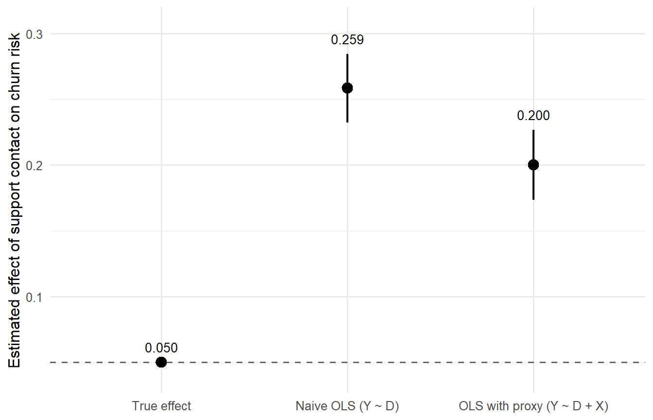
The algebra is exact but cold. A simulation makes the bias tactile. We build a world in which the true causal effect of support contact on churn risk is small and known, `true_beta = 0.05`. A latent frustration variable $U$ drives both support contact $D$ and churn risk $Y$, and an observed proxy $X$ (say, the count of past complaints logged in the CRM) is correlated with $U$ but is not $U$ itself.
```{r}
#| label: fig-ovb-simulation
#| fig-cap: "Naive OLS overstates the true causal effect of support contact on churn risk by more than a factor of five. Adding a covariate correlated with the true confounder shrinks the bias and narrows the confidence interval, but the point estimate remains far from the truth."
#| fig-width: 7
#| fig-height: 4.5
set.seed(2026)

n <- 5000
true_beta <- 0.05
gamma     <- 0.5

# Latent frustration: unobserved by the analyst
U <- rnorm(n)

# Support-contact intensity: frustrated customers contact support more
D <- 0.6 * U + rnorm(n)

# Observed proxy correlated with U but not equal to U
X <- 0.7 * U + rnorm(n)

# Churn-risk score; true causal effect of D is small and positive
Y <- true_beta * D + gamma * U + rnorm(n)

df_churn_sim <- data.frame(Y = Y, D = D, X = X)

# Naive OLS: Y on D alone
fit_naive    <- lm(Y ~ D,     data = df_churn_sim)
beta_naive   <- unname(coef(fit_naive)["D"])
se_naive     <- summary(fit_naive)$coefficients["D", "Std. Error"]

# Partially controlled OLS: Y on D plus observed proxy X
fit_partial  <- lm(Y ~ D + X, data = df_churn_sim)
beta_partial <- unname(coef(fit_partial)["D"])
se_partial   <- summary(fit_partial)$coefficients["D", "Std. Error"]

results <- data.frame(
  specification = factor(
    c("True effect", "Naive OLS (Y ~ D)", "OLS with proxy (Y ~ D + X)"),
    levels = c("True effect", "Naive OLS (Y ~ D)", "OLS with proxy (Y ~ D + X)")
  ),
  estimate = c(true_beta, beta_naive, beta_partial),
  se       = c(NA, se_naive, se_partial)
)

ggplot(results, aes(x = specification, y = estimate)) +
  geom_hline(yintercept = true_beta, linetype = "dashed", color = "grey40") +
  geom_pointrange(
    aes(ymin = estimate - 1.96 * se, ymax = estimate + 1.96 * se),
    size = 0.7, linewidth = 0.8, na.rm = TRUE
  ) +
  geom_text(
    aes(
      label = sprintf("%.3f", estimate),
      y = estimate + 1.96 * ifelse(is.na(se), 0, se)
    ),
    vjust = -1, size = 3.6
  ) +
  scale_y_continuous(expand = expansion(mult = c(0.10, 0.15))) +
  labs(
    x = NULL,
    y = "Estimated effect of support contact on churn risk"
  ) +
  theme_minimal(base_size = 12)
```
The naive OLS estimate lands near 0.27, more than five times the truth, and the direction of the bias is exactly what the formula predicts: $\gamma > 0$ and $\operatorname{Cov}(D, U) > 0$ deliver a positive bias, so the estimator overstates $\beta$. Adding the observed proxy $X$ pulls the point estimate down toward 0.21, closer to the truth but still meaningfully above it, because $X$ is a noisy stand-in for $U$ and residual selection remains. The confidence interval also tightens, giving a false sense of precision around the wrong number. The gap between the middle and right point in the figure is the story of this section: controlling for something related to the confounder is not the same as controlling for the confounder, and the residual bias does not vanish with more data. Doubling $n$ tightens the interval around the biased estimate. It does not move the estimate.
::: {.callout-warning title="Controlling for the wrong thing"}
Adding a covariate that is correlated with the true unobserved confounder can shrink the bias without eliminating it, leaving an estimate that looks disciplined but is still systematically wrong. This is more dangerous than an obviously naive comparison, because the specification now carries the visual signature of rigor, controls, standard errors, and a nicely behaved table, while quietly answering a question no one asked. A smaller bias is not a zero bias, and a model with controls is not a causal model by virtue of having them.
:::
The way out is not a better control variable. It is a variable that is correlated with $D$ but is guaranteed, by its own construction or origin, to have no relationship with $U$, and Section III turns that requirement into three precise, checkable conditions.
## Section III. The Three Conditions: Relevance, Exclusion, and Independence
Return to the Vietnam draft lottery from Section I. What made that lottery number a valid instrument for the causal effect of military service on later earnings? The answer is not one property but three, each doing a separate job, and every later section of this post refers back to them by name. Let $Z$ denote the instrument (lottery number), $D$ the treatment (veteran status), $Y$ the outcome (earnings), and $U$ the unobserved confounder that entangled $D$ and $Y$ in the OLS analysis of Section II. In potential outcomes notation, $Y_i(d)$ is the outcome individual $i$ would experience under treatment value $d$, and $D_i(z)$ is the treatment status individual $i$ would take under instrument value $z$.
### Relevance
The first condition is the most mechanical. The instrument must actually move the treatment:
$$\text{Cov}(Z, D) \neq 0.$$
In plain language, changes in $Z$ must be associated with changes in the probability of receiving $D$, and by an amount large enough to be estimated with precision in finite samples. For the draft lottery, relevance is visible in the raw tabulation. Among men born in 1950, those with random sequence numbers at or below the eligibility cutoff of 195 served at a rate of 35.3 percent, compared with 19.3 percent for those above the cutoff, a gap of roughly 16 percentage points (Angrist, Imbens & Rubin, 1996, Table 2). The lottery moved military service, and it moved it by a lot. Section VI takes up the weak-instrument diagnostics that formalize what "by a lot" has to mean in finite samples.
Relevance is the only one of the three conditions that can be checked directly in the data. You regress $D$ on $Z$, and you look at the coefficient. This is why every serious IV paper reports the first-stage results prominently.
### Exclusion restriction
The second condition is where the real intellectual work begins. The exclusion restriction states that the instrument affects the outcome only through its effect on the treatment, with no direct path from $Z$ to $Y$. In potential outcomes notation (Imbens & Angrist, 1994; Angrist, Imbens & Rubin, 1996), where $Y_i(z, d)$ denotes the outcome individual $i$ would experience if assigned instrument value $z$ and treatment status $d$,
$$Y_i(z, d) = Y_i(d) \quad \text{for all } z.$$
A person's outcome depends only on the treatment they actually receive, not on which value of the instrument happened to assign them to that treatment level. Holding $d$ fixed, changing $z$ from $0$ to $1$ leaves the potential outcome unchanged. For the draft lottery, this means a lottery number can affect lifetime earnings only by changing whether someone served. A low number is just a number; it has no biological or economic effect of its own, so it cannot directly alter health, family connections, or employer preferences. The outcome channel runs exclusively through military service.
Exclusion — unlike relevance — is almost never directly testable. It is a statement about the absence of a causal path that runs through the very unobserved factors the instrument is meant to sidestep. You cannot regress $Y$ on $Z$ controlling for $D$ and interpret the residual as a test of exclusion, because that regression also absorbs variation driven by $U$. Exclusion is a matter of institutional knowledge and argument, not a number you compute from a regression table. Section VII takes up falsification checks that can rule out specific violations without ever confirming the assumption itself.
### Independence
The third condition, often called the "as-if random" assumption, requires that the instrument itself be uncorrelated with anything that determines either the outcome or the treatment. Formally,
$$Z_i \perp (Y_i(d), D_i(z)) \quad \text{for all } d, z,$$
where the symbol $\perp$ denotes statistical independence: knowing the value of $Z_i$ carries no information about the distribution of the potential outcomes $Y_i(d)$ or the potential treatment status $D_i(z)$. The instrument must be independent of both. The joint independence with $D_i(z)$ is the stronger version required to identify the local average treatment effect, which we develop in Section V.
Distinguish this carefully from exclusion, because conflating the two is one of the most common errors in informal treatments of instrumental variables. Exclusion says there is no direct arrow from $Z$ to $Y$. Independence says $Z$ itself is not a consequence of the confounder $U$ that points to both $D$ and $Y$, the same $U$ from the churn simulation in Section II, now named in the general case. An instrument can satisfy exclusion (no direct effect on $Y$) while violating independence (correlated with $U$). Had the draft lottery been quietly manipulated so that men from wealthier families received lower numbers, the lottery number would carry information about family background, a determinant of later earnings, even if the number itself had no direct effect on anything. Relevance is a fact about the data. Exclusion is a fact about the world. Independence is a fact about how the instrument was generated.
In the draft lottery, independence holds because the numbers were drawn from a physical randomization device: the Selective Service assigned a random sequence number to each date of birth without regard to any personal characteristic. The assignment mechanism had no connection to ambition, family background, or health, the latent variables collected in $U$.
### Putting the three together
The full causal structure can be described in a single sentence. $Z$ points to $D$, $D$ points to $Y$, and a confounder $U$ points to both $D$ and $Y$. Critically, there is no arrow from $Z$ to $Y$ directly (exclusion), and no arrow from $U$ to $Z$ (independence). Relevance guarantees that the arrow from $Z$ to $D$ is strong enough to detect.
The asymmetry across the three conditions is the single most important thing to understand about how IV analyses are actually evaluated by referees and by careful readers. Relevance is checkable in the data. Exclusion and independence are not: they are assumptions the researcher must argue for using institutional knowledge, and everyone reading the paper knows it. As Angrist and Pischke (2009) put it, the credibility of an IV strategy rests almost entirely on the persuasiveness of these two arguments, not on the size of the first-stage $F$-statistic.
A brief counter-example sharpens the definitions. Consider using rainfall on election day as an instrument for voter turnout when studying the effect of turnout on local policy outcomes. Rainfall plausibly satisfies relevance, since bad weather demonstrably lowers turnout, and it may satisfy independence as well. But it can violate exclusion if rainfall also affects policy outcomes directly through a separate channel, for instance by depressing agricultural output in rural districts on the day of the vote and thereby shifting local economic conditions through a path that has nothing to do with who showed up at the polls. The instrument is not invalidated by a weak first stage; it is invalidated by a forbidden causal channel.
With the three conditions precisely defined, the next section shows how they combine, algebraically, into an actual estimator. We start with the simplest possible case, a single binary instrument and a single binary treatment.
::: {.callout-tip title="The one condition you can actually test"}
Relevance is checkable with a first-stage regression of $D$ on $Z$, the subject of Section VI. Exclusion and independence are not; they require institutional knowledge and argument. Most disputes over whether an IV study is credible are really disputes about the latter two, not about the size of the first stage.
:::
## Section IV. From Assumptions to Estimand: Deriving 2SLS and the Wald Estimator
A binary instrument $Z_i \in \{0,1\}$ records whether individual $i$ received a lottery number below the eligibility cutoff. A binary treatment $D_i \in \{0,1\}$ records whether $i$ actually served in the military. The outcome $Y_i$ is a later-life measure such as log annual earnings. Relevance, exclusion, and independence (as established in Section III) are assumed to hold throughout. From here on, the task is mechanical: turn those three assumptions into a formula.
### The Wald estimator
Start with the **reduced-form** contrast, the difference in average outcomes across the two instrument groups:
$$
E[Y_i \mid Z_i = 1] - E[Y_i \mid Z_i = 0].
$$
This quantity is directly estimable from the data. It tells us how much earnings differ, on average, between those the lottery pushed toward service and those it did not. It does not, on its own, tell us the effect of service.
To connect the reduced form to the causal parameter of interest, invoke the exclusion restriction. Under exclusion, $Z_i$ affects $Y_i$ only through $D_i$, so we can write $Y_i = Y_i(0) + \beta D_i$ under a constant-effect model, where $\beta$ is the effect we want to recover. Substituting into the reduced form,
$$
\begin{aligned}
E[Y_i \mid Z_i = 1] - E[Y_i \mid Z_i = 0]
&= E[Y_i(0) \mid Z_i=1] - E[Y_i(0) \mid Z_i=0] \\
&\quad + \beta\big(E[D_i \mid Z_i=1] - E[D_i \mid Z_i=0]\big).
\end{aligned}
$$
Independence now does the heavy lifting. Because $Z_i$ is independent of the potential outcomes, $E[Y_i(0) \mid Z_i=1] = E[Y_i(0) \mid Z_i=0]$ and the first two terms cancel exactly. What remains is the treatment effect scaled by a difference in average treatment status:
$$
E[Y_i \mid Z_i = 1] - E[Y_i \mid Z_i = 0]
=
\beta\big(E[D_i \mid Z_i = 1] - E[D_i \mid Z_i = 0]\big).
$$
The bracketed quantity is the **first stage**, the difference in the probability of being treated between the two instrument groups. Under relevance, it is non-zero. Divide both sides by it, replace population expectations by sample means, and solve for $\beta$:
$$
\hat{\beta}_{IV}
=
\frac{E[Y_i \mid Z_i = 1] - E[Y_i \mid Z_i = 0]}{E[D_i \mid Z_i = 1] - E[D_i \mid Z_i = 0]}.
$$
This is the **Wald estimator** (Wald, 1940). The numerator is the reduced form, how much the instrument moves the outcome. The denominator is the first stage, how much the instrument moves the treatment, and it is the empirical counterpart of the relevance condition from Section III. In one sentence: the Wald estimator takes the effect of the instrument on the outcome and rescales it by how much of the treatment the instrument was actually responsible for changing.
The rescaling is not cosmetic. A reduced-form effect of $-0.005$ on log earnings means very different things depending on whether the instrument moves service by 50 percentage points or by 5. If the instrument barely moves the treatment, the denominator shrinks toward zero and the ratio explodes, a foreshadowing of the weak-instrument problem we return to in Section VI.
### Keeping only the variation we trust
The algebra shows how the Wald estimator works. Chris Said (2021) offers an informal but rigorous companion that makes 2SLS click for most first-time readers by framing the problem as a variance decomposition of the endogenous treatment.
Think of the variation in $D$ as splitting into two pieces. One piece is the part of $D$ that the instrument $Z$ can explain, the variation in treatment that moves in lockstep with lottery draws. The other piece is everything else, the part of $D$ that varies for reasons the instrument does not touch, including whatever is entangled with the unobserved confounder $U$ from Section II. The first piece is clean by construction: because $Z$ is independent of $U$, any variation in $D$ that tracks $Z$ cannot be tracking $U$. The second piece is contaminated.
Two-stage least squares operationalizes exactly this split. In a first-stage regression, we predict $D$ from $Z$ and keep only the fitted values $\hat{D}_i$. In a second-stage regression, we use $\hat{D}$ in place of $D$. The fitted values $\hat{D}_i$ — by construction — carry only the part of the treatment explained by the instrument. Because $\hat{D}$ is a function of $Z$ alone, and $Z$ is independent of $U$ by the independence condition, $\hat{D}$ inherits none of the correlation with $U$ that made the original $D$ endogenous. The endogeneity is not purged by controlling for the confounder, which we cannot observe; it is purged by discarding the part of $D$ that could plausibly be carrying it.
OLS uses all of the variation in $D$. 2SLS uses only the part it can trust.
### From Wald to 2SLS with covariates
The Wald formula assumes there are no other variables to condition on. In practice, we often want to include a vector of exogenous controls $X_i$, whether for precision, to defend exclusion within strata, or because the instrument is only as-good-as-randomly-assigned conditional on $X_i$. Two-Stage Least Squares generalizes Wald to these cases. With one endogenous regressor $D_i$, one instrument $Z_i$, and a vector of exogenous controls $X_i$, the two stages are:
$$
\text{First stage:}\quad D_i = \pi_0 + \pi_1 Z_i + \pi_2' X_i + \nu_i,
$$
$$
\text{Second stage:}\quad Y_i = \beta_0 + \beta_1 \hat{D}_i + \beta_2' X_i + \epsilon_i,
$$
where $\hat{D}_i$ is the fitted value from the first stage, $X_i$ appears in both stages, $\pi_1$ measures instrument strength conditional on $X_i$, and $\beta_1$ is the causal parameter of interest. The instrument $Z_i$ can be a scalar or a vector; when there are more instruments than endogenous regressors, the model is over-identified, and 2SLS combines the available instruments through the first-stage projection (Angrist and Pischke, 2009, Ch. 4).
The connection between the two formulas is precise, and it is worth stating carefully because it is often mis-stated. In the just-identified case with one instrument, one endogenous regressor, and no covariates, 2SLS is numerically identical to the Wald estimator. When exogenous covariates $X_i$ are added, 2SLS equals the Wald estimator computed on residuals, after $X_i$ has been partialled out of $Z_i$, $D_i$, and $Y_i$ by OLS. This is Frisch-Waugh-Lovell applied to the just-identified IV setting. The equivalence does not extend to over-identified models: with multiple instruments, 2SLS becomes a weighted combination of instrument-specific Wald ratios, with weights determined by the first-stage covariance structure, not a single Wald ratio. For the everyday one-instrument, one-treatment case, Wald and 2SLS are two ways of writing the same number.
### A worked numerical example
To make the arithmetic concrete, return to the draft lottery framing with illustrative summary statistics. These are not the actual Angrist (1990) estimates, they are chosen to be plausible and to keep the arithmetic clean.
Suppose being assigned a low lottery number raises the probability of military service by 15 percentage points:
$$
E[D_i \mid Z_i=1] - E[D_i \mid Z_i=0] = 0.15.
$$
Suppose those same men have log annual earnings lower by 0.0045 on average:
$$
E[Y_i \mid Z_i=1] - E[Y_i \mid Z_i=0] = -0.0045.
$$
The implied Wald estimate is
$$
\hat{\beta}_{IV} = \frac{-0.0045}{0.15} = -0.03.
$$
In plain language, for the men whose service status was actually shifted by their lottery number, military service reduced subsequent earnings by approximately 3%. The reduced-form contrast is small (0.45 log points) because most men who served would have served regardless of their lottery number, and many men with low numbers avoided service altogether. The Wald estimator rescales that small reduced-form contrast by the 15-percentage-point first stage to recover a much larger implied treatment effect. A tiny reduced form is not a tiny effect once it has been properly rescaled.
### Simulation: recovering a known true effect
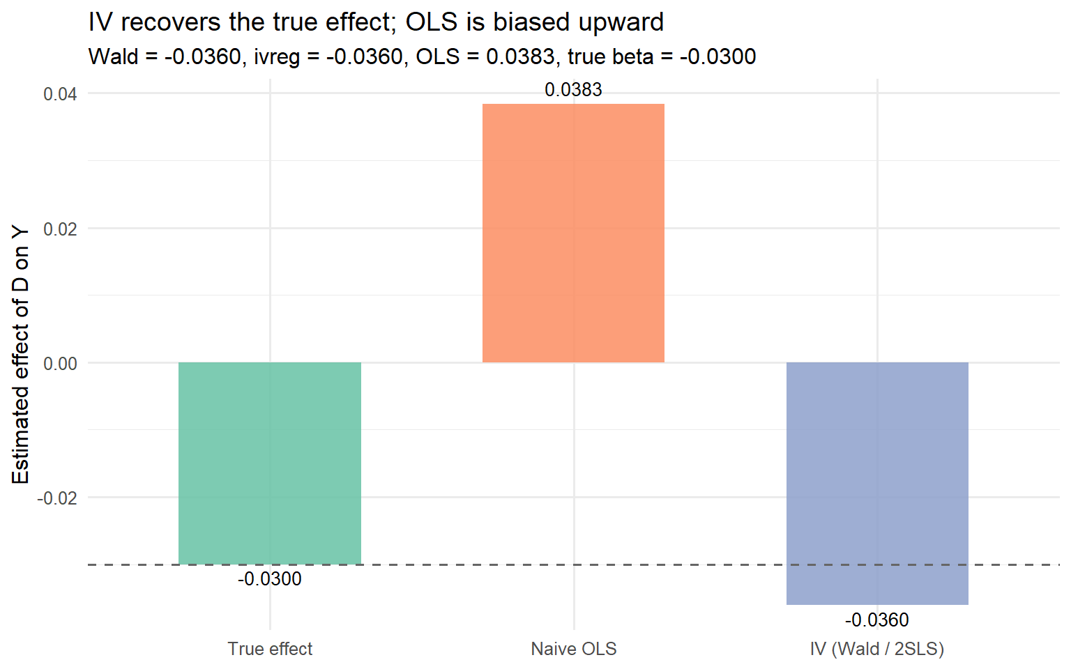
The following chunk simulates a binary-instrument, binary-treatment dataset satisfying the three conditions from Section III, computes the Wald estimator by hand, refits the same model with `ivreg()`, contrasts both against a naive OLS, and plots the three estimates against the known truth.
```{r}
#| label: fig-wald-vs-ols
#| fig-cap: "Naive OLS is biased upward by the confounder $U$; IV (Wald and 2SLS coincide in the just-identified case) recovers the true effect true_beta = -0.03 within Monte Carlo error. The dashed line marks the truth."
#| message: false
#| warning: false
library(ivreg)
library(dplyr)
library(ggplot2)

set.seed(2026)

n <- 10000
true_beta <- -0.03

# Confounder U enters both D and Y (this is the endogeneity from Section II).
# Instrument Z is randomly assigned and enters only D (exclusion + independence).
U <- rnorm(n)
Z <- rbinom(n, 1, 0.5)

# Binary treatment: probability of service depends on Z (first stage) and U (endogeneity)
p_D <- pnorm(-0.3 + 0.7 * Z + 0.5 * U)
D   <- rbinom(n, 1, p_D)

# Outcome: linear in D and U, with a known true effect and low noise
Y <- true_beta * D + 0.10 * U + rnorm(n, sd = 0.05)

df_draft_sim <- tibble(Y = Y, D = D, Z = Z, U = U)

# Wald estimator by hand: reduced form divided by first stage
rf   <- mean(df_draft_sim$Y[df_draft_sim$Z == 1]) -
        mean(df_draft_sim$Y[df_draft_sim$Z == 0])
fs   <- mean(df_draft_sim$D[df_draft_sim$Z == 1]) -
        mean(df_draft_sim$D[df_draft_sim$Z == 0])
wald_hat <- rf / fs

# 2SLS via the ivreg formula interface: Y ~ D | Z
iv_fit <- ivreg(Y ~ D | Z, data = df_draft_sim)
iv_hat <- unname(coef(iv_fit)["D"])

# Naive OLS of Y on D alone, for contrast
ols_fit <- lm(Y ~ D, data = df_draft_sim)
ols_hat <- unname(coef(ols_fit)["D"])

cat("First stage       :", round(fs, 4), "\n",
    "Reduced form      :", round(rf, 4), "\n",
    "Wald (by hand)    :", round(wald_hat, 4), "\n",
    "IV (ivreg)        :", round(iv_hat, 4), "\n",
    "Naive OLS         :", round(ols_hat, 4), "\n",
    "True beta         :", true_beta, "\n")
df_plot <- tibble(
  estimator = factor(
    c("True effect", "Naive OLS", "IV (Wald / 2SLS)"),
    levels = c("True effect", "Naive OLS", "IV (Wald / 2SLS)")
  ),
  estimate  = c(true_beta, ols_hat, iv_hat)
)

ggplot(df_plot, aes(x = estimator, y = estimate, fill = estimator)) +
  geom_col(width = 0.6, alpha = 0.85) +
  geom_hline(yintercept = true_beta, linetype = "dashed", color = "grey40") +
  geom_text(aes(label = sprintf("%.4f", estimate)),
            vjust = ifelse(df_plot$estimate < 0, 1.4, -0.6),
            size = 3.6) +
  scale_fill_brewer(palette = "Set2") +
  labs(
    x = NULL,
    y = "Estimated effect of D on Y",
    title = "IV recovers the true effect; OLS is biased upward",
    subtitle = sprintf(
      "Wald = %.4f, ivreg = %.4f, OLS = %.4f, true beta = %.4f",
      wald_hat, iv_hat, ols_hat, true_beta
    )
  ) +
  theme_minimal(base_size = 12) +
  theme(legend.position = "none")
```
Three things are worth noticing. First, the hand-computed Wald estimate and the `ivreg` coefficient agree to four decimal places, confirming the just-identified equivalence numerically. Second, both recover `true_beta = -0.03` within Monte Carlo error. Third, the naive OLS estimate is biased in the positive direction, exactly the failure mode Section II warned about: because $D$ and $U$ are positively correlated by construction and $U$ enters $Y$ positively, OLS attributes to $D$ part of the earnings variation that actually belongs to $U$, masking the negative treatment effect.
::: {.callout-note title="Why the first stage matters twice"}
The first-stage coefficient does two jobs at once. It is the denominator of the Wald estimator, so its magnitude directly scales the point estimate: a small first stage turns a small reduced form into a large and unstable IV coefficient. Its statistical strength, previewed here and formalized in Section VI, also determines whether the entire IV estimate can be trusted at all; a first stage that is not merely small but noisy relative to sampling error is the definition of a weak instrument, and weak instruments can bias 2SLS more severely than the OLS it was meant to fix.
:::
The Wald estimator and 2SLS answer the question "what is the effect of $D$ on $Y$", but under the conditions maintained so far, the answer is not necessarily the effect for everyone. The next section defines precisely whose effect this is, and why the parameter identified by IV under one-sided noncompliance and heterogeneous effects is called a Local Average Treatment Effect.
## Section V. What IV Actually Estimates: The LATE and Its Discontents
Among the men whose Vietnam draft lottery number determined whether they were called to serve, not every one of them was actually persuadable by the lottery. Some would have served regardless of their number, because they intended to enlist anyway. Others would have avoided service regardless, because they had deferments, medical exemptions, family connections, or the means to leave the country. The lottery only shifted the behavior of a specific subset. The IV estimate from Section IV is therefore not the average effect of military service on earnings for all draft-eligible men. It is the average effect for exactly that subset. This is the central complication of instrumental variables: it does not generally recover the Average Treatment Effect (ATE). It recovers a different, more specific quantity, and the rest of this section defines precisely what that quantity is and why it matters for anyone acting on the estimate.
### The four latent types
Following Imbens and Angrist (1994) and Angrist, Imbens and Rubin (1996), let $Z_i \in \{0, 1\}$ denote the instrument and let $D_i(1)$ and $D_i(0)$ denote individual $i$'s potential treatment status when $Z_i = 1$ and $Z_i = 0$, respectively. In the draft lottery setting, $D_i(1)$ is whether man $i$ would serve if his number made him draft-eligible, and $D_i(0)$ is whether he would serve if it did not. Both potential statuses exist for every individual, but only one of them is ever observed, the one associated with the instrument value actually realized. Every individual in the population falls into exactly one of four latent types:
- **Compliers**, with $D_i(1) = 1$ and $D_i(0) = 0$: they take the treatment only if assigned the instrument, meaning they would serve if drafted and would not serve otherwise.
- **Always-takers**, with $D_i(1) = D_i(0) = 1$: they take the treatment regardless of the instrument, meaning they would serve whether or not they were drafted; career volunteers fall into this group.
- **Never-takers**, with $D_i(1) = D_i(0) = 0$: they never take the treatment regardless of the instrument, meaning they would avoid service under any lottery number; men with hard deferments or those willing to leave the country fall into this group.
- **Defiers**, with $D_i(1) = 0$ and $D_i(0) = 1$: they do the opposite of what the instrument encourages, meaning they would serve if not drafted and would refuse if drafted.
Type membership is unobservable, because we only ever see the treatment status corresponding to each individual's realized instrument value. Making progress requires an additional assumption that pins down which of these types can plausibly coexist in the population.
### Monotonicity
The **monotonicity** assumption, introduced by Imbens and Angrist (1994), requires that $D_i(1) \geq D_i(0)$ for all $i$. In plain terms, no one in the population is pushed away from treatment by the instrument. Equivalently, there are no defiers. The instrument may leave some individuals unchanged (always-takers and never-takers) and may push others toward treatment (compliers), but it cannot push anyone in the opposite direction.
What monotonicity buys is the absence of canceling flows. Without it, the instrument could nudge some men into service and other men out of it, with the two behavioral responses partially offsetting in aggregate, so the Wald ratio would average over opposing movements and lose its clean interpretation as a per-person effect. Unlike relevance, monotonicity is not directly testable from the data; it sits on the argued side of the testable-versus-argued asymmetry established in Section III, alongside exclusion and independence, and must be defended on institutional or behavioral grounds.
### The LATE theorem
Under relevance, exclusion, independence, and monotonicity, the Wald estimator from Section IV converges to
$$E\!\left[Y_i(1) - Y_i(0) \,\middle|\, D_i(1) > D_i(0)\right],$$
the average treatment effect for compliers, known as the **Complier Average Causal Effect (CACE)** or, equivalently, the **Local Average Treatment Effect (LATE)**. The conditioning event $D_i(1) > D_i(0)$ picks out exactly the complier subpopulation, since under monotonicity compliers are the only individuals whose treatment status responds to the instrument.
The intuition for why only compliers contribute is mechanical. Always-takers have the same treatment status under either value of the instrument, so their treated outcomes appear symmetrically on both instrument arms and cancel from the numerator of the Wald ratio. Never-takers cancel from the other side, with their untreated outcomes appearing under both instrument values. Defiers are ruled out by assumption. Only compliers switch treatment status, from $D_i(0) = 0$ to $D_i(1) = 1$, so only their outcome differences survive in the numerator, and only their share of the population appears in the denominator. The Wald ratio is a ratio of complier-generated quantities and it identifies a complier-specific effect.
### Why this matters in practice
The LATE from the draft lottery describes the effect of military service on earnings for men who served because they were drafted and would not have served otherwise. It says nothing directly about always-takers, the men who would have volunteered regardless, even though a policymaker asking "should we reinstate the draft" or "what is the effect of military service in general" might actually care most about a different population.
The same treatment, estimated with a different instrument, can identify the LATE for an entirely different complier population and can produce a different numerical answer, without either estimate being wrong. A draft lottery identifies the effect for draft-marginal men. An instrument based on enlistment bonuses would identify it for bonus-marginal men. A proximity-to-base instrument would identify a third population. None of these is the ATE, and none of them contradicts the others. This is not an inconsistency, it is a feature of what each specific instrument identifies, and the practitioner's job is to know which population the estimate speaks about.
### The honest resolution: better LATE than nothing
The standard critique of the LATE is that it is "too local" to guide policy. Imbens (2010) makes the opposite case fairly. A LATE for a well-defined, policy-relevant complier population is often exactly what a decision-maker needs. The individuals at the margin of being affected by a specific proposed policy change are precisely the compliers for the instrument that the policy itself would manipulate, so the LATE for that instrument is the directly decision-relevant quantity. An ATE that averages in always-takers, whose behavior would not change under the policy anyway, is for that specific decision less informative than the LATE, not more. "Local" is a liability only when the local population is not the one the policy acts on, and an asset when it is.
### A forward pointer on multiple and continuous instruments
When several instruments are combined in a single 2SLS specification, or when the instrument or treatment is continuous, the aggregation of complier populations becomes considerably more complex. Under treatment effect heterogeneity, the 2SLS estimand can place negative weights on some complier groups' effects, so the resulting estimate need not correspond to any well-defined causal effect for a real population (Mogstad, Torgovitsky and Walters, 2021). The clean single-instrument LATE interpretation is a special case, not a generic guarantee, and the reader who plans to combine instruments in one specification should treat that section of the literature as required reading rather than optional.
### Bridge to Section VI
Everything from Section III onward has assumed the instrument is strong enough to be useful in the first place. The next section shows what happens when it is not, and how to check before trusting any of this.
::: {.callout-warning title="Ask what population your instrument speaks for"}
Before reporting or acting on any IV estimate, you should be able to state, in one plain sentence, who the compliers plausibly are for your specific instrument. If you cannot, the number you are reporting is a LATE for an unnamed population, and any decision built on it inherits that ambiguity. Failing to name the complier population is the single most common way IV results get misinterpreted in applied work.
:::
## Section VI. Is Your Instrument Actually Strong? Weak Instrument Diagnostics in Practice
Picture the moment an analyst finishes running `ivreg()` on a new dataset. The coefficient on the endogenous treatment prints with a plausible sign, a standard error small enough to give a $p$-value under 0.05, and a 95% confidence interval that excludes zero. Everything on the printout looks like a clean identification result. Whether that number can actually be trusted depends on something the printout does not show: how hard the instrument $Z$ was pushing on the treatment $D$ in the first stage. Sections IV and V treated the first-stage coefficient as a positive number and moved on. This section asks what happens when that assumption barely holds.
### The mechanism: dividing by a number close to zero
Recall the Wald estimator from Section IV,
$$\hat{\beta}_{\text{IV}} \;=\; \frac{\widehat{\text{Cov}}(Y, Z)}{\widehat{\text{Cov}}(D, Z)}.$$
The denominator is the empirical first-stage relationship. When $Z$ genuinely shifts $D$, that denominator sits well away from zero and small perturbations barely move the ratio. When $Z$ shifts $D$ only weakly, the denominator is a small number estimated with noise, and every draw of the data produces a wildly different divisor. The point estimate then swings erratically from sample to sample and can flip sign entirely.
This is not a small-sample nuisance that vanishes with $n$ in the usual way. It is a property of the ratio structure of the estimator itself. Dividing by a quantity close to zero remains unstable no matter how large the sample gets, *unless the first-stage relationship strengthens with it*. If the true first-stage coefficient is small and fixed, more data only narrows the distribution of the denominator around a small number, which is precisely the regime where the ratio behaves badly.
### The formal consequence: standard inference breaks
Staiger and Stock (1997) formalized this by modelling the first-stage coefficient as local-to-zero, shrinking with the sample size so that the signal-to-noise ratio stays bounded. Under that asymptotic device, the sampling distribution of the 2SLS estimator does not converge to the normal distribution ordinary asymptotic theory promises. It is skewed, can be badly centred relative to the true parameter, and, most damagingly for practice, the standard errors reported by conventional software understate the true dispersion.
The warning a decision-maker can act on: a weak instrument does not merely give an imprecise estimate with wider intervals. It gives a *misleading* one. The 95% confidence interval printed next to the coefficient covers the true parameter far less than 95% of the time, and reporting it as if it were valid overstates the credibility of the finding.
### The classical diagnostic: first-stage F
The practical response, also from Staiger and Stock (1997), is to inspect the first-stage regression directly. Using the notation from Section IV,
$$D_i \;=\; \pi_0 + \pi_1 Z_i + \pi_2' X_i + \nu_i,$$
the first-stage F-statistic tests $H_0: \pi_1 = 0$ (or, with multiple excluded instruments, the joint null that all their coefficients are zero). Intuitively, it asks how much of the variation in $D$ the instrument reliably explains once controls are partialled out. This is the relevance condition from Section III, dressed up as a hypothesis test.
The rule of thumb that entered applied practice through Staiger and Stock (1997) is: treat a first-stage F below 10 as a warning sign of a weak instrument. The number is not arbitrary, it was chosen as a rough boundary beyond which the local-to-zero asymptotics start to behave reasonably.
Stock and Yogo (2005) made this rigorous. They derived critical values for weak-instrument tests that depend on (i) how much bias, relative to OLS, a researcher is willing to tolerate, (ii) the number of excluded instruments, and (iii) the number of endogenous regressors. Their tables show that F > 10 corresponds, in the single-endogenous-regressor case, roughly to a worst-case 2SLS bias of at most 10% of the OLS bias. That is a specific, calibrated target, not a round number chosen for convenience.
### The modern complication: bias control is not inference control
Here the story turns uncomfortable. Lee, McCrary, Moreira and Porter (2022) show that the classical F > 10 threshold, while defensible as a bias-control diagnostic, is far too permissive for the object practitioners actually care about most, the validity of the usual $t$-ratio and the confidence interval built from it. Their result, derived for the just-identified case using the standard 2SLS $t$-ratio at the 5% level, implies that a first-stage F on the order of 104.7 is needed before the conventional 1.96 critical value delivers correct size. That is roughly an order of magnitude above the familiar rule of thumb. The claim is scoped to $t$-ratio inference at conventional levels, not offered as a universal replacement for F > 10 in every setting.
The intuition is that bias and inference validity are different objects. An estimator can be nearly unbiased on average while still having a sampling distribution too irregular, too skewed or too heavy-tailed, for a normal-based confidence interval to have correct coverage. Passing a bias test does not certify that the $t$-ratio is normal.
### A more robust diagnostic
The classical F-statistic assumes homoskedastic, serially uncorrelated errors, an assumption routinely violated in applied work. Montiel Olea and Pflueger (2013) introduced an *effective F-statistic* that adjusts the classical statistic to remain valid under heteroskedasticity, autocorrelation, and clustering. In most modern applied settings, where cluster-robust standard errors are the default, this is the diagnostic that should actually be reported. Andrews, Stock and Sun (2019) provide a practical review and confirm, on a survey of AER papers, that weak instruments remain a live problem in published work.
The uncomfortable empirical fact is that many of the "classic" instruments taught in graduate textbooks have failed even the permissive F > 10 threshold when scrutinised on the original data. The quarter-of-birth instruments of Angrist and Krueger (1991), which Section VIII dissects, are the canonical case, and Bound, Jaeger and Baker (1995) is the reference for how badly the first stage there behaves once you look at it closely. The Vietnam draft lottery from Section I is one of the rare instruments strong enough to survive this section without qualification. Most are not.
### What to do when your instrument is weak
Three responses, in order of preference:
1. **Prune your instruments.** If you are using several excluded instruments and the joint F is weak, retain only the strongest one. Overidentification is not free, adding weak instruments can drag the effective strength down and can make finite-sample bias worse.
2. **Use weak-instrument-robust inference.** The Anderson–Rubin test and related procedures produce confidence sets whose coverage is correct regardless of instrument strength. They are more conservative when instruments are strong and can produce unbounded or empty sets when instruments are weak, which is the *honest* signal that the data cannot identify the parameter. These are covered in the advanced references and are the right tool when strength is borderline.
3. **Report and decline.** The most honest response, if the first stage is genuinely weak and no stronger instrument is available, is to report the diagnostics, decline to draw a causal conclusion from this instrument, and be explicit about the limitation. A point estimate that cannot be trusted is worse than no point estimate at all.
### Simulation: strong vs. weak first stage, same true effect
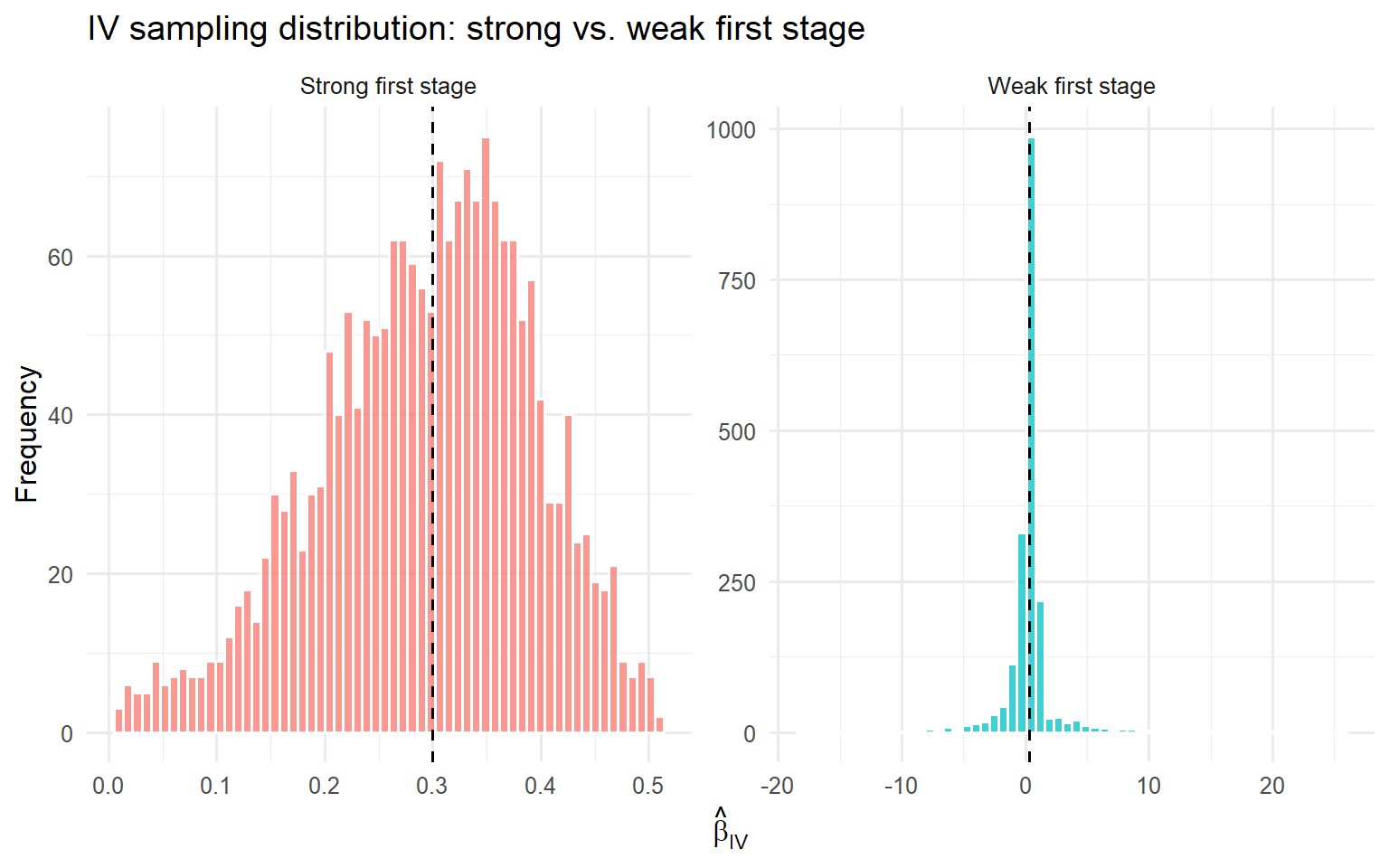
The following simulation isolates first-stage strength as the only difference between two data-generating processes. Everything else, the sample size, the confounding structure, and the true structural effect $\beta = 0.3$, is held fixed. The structural error $u$ and the first-stage error $v$ are correlated with $\rho = 0.9$, which is the source of endogeneity that motivates using IV in the first place.
```{r}
#| label: fig-weak-iv-sampling
#| fig-cap: "Sampling distribution of the IV estimator across 2,000 replications under a strong first stage ($\\pi_1 = 0.70$) and a weak first stage ($\\pi_1 = 0.10$). Both scenarios share the same true structural effect $\\beta = 0.3$ (dashed line), the same sample size, and the same error-correlation structure. The weak-instrument distribution is visibly wider, skewed, and shifted away from the truth; the strong-instrument distribution is tight and approximately symmetric around $\\beta$."
#| fig-width: 8
#| fig-height: 5
set.seed(2026)

n            <- 200
n_sims       <- 2000
true_beta    <- 0.3
pi_strong    <- 0.70   # strong first stage
pi_weak      <- 0.10   # weak first stage
rho          <- 0.9    # correlation between structural and first-stage errors

simulate_iv <- function(pi_first, n, true_beta, rho) {
  Z  <- rnorm(n)
  e1 <- rnorm(n)
  e2 <- rnorm(n)
  u  <- e1                                      # structural error
  v  <- rho * e1 + sqrt(1 - rho^2) * e2         # first-stage error, cor(u, v) = rho
  D  <- pi_first * Z + v
  Y  <- true_beta * D + u
  dat <- data.frame(Y = Y, D = D, Z = Z)

  # first-stage F (classical, homoskedastic)
  fs   <- lm(D ~ Z, data = dat)
  F_fs <- summary(fs)$fstatistic["value"]

  # 2SLS via ivreg, with nominal 95% CI built from the printed SE
  iv   <- ivreg(Y ~ D | Z, data = dat)
  co   <- summary(iv)$coefficients
  bhat <- co["D", "Estimate"]
  se   <- co["D", "Std. Error"]

  ci_lo   <- bhat - 1.96 * se
  ci_hi   <- bhat + 1.96 * se
  covered <- (ci_lo <= true_beta) & (true_beta <= ci_hi)

  c(F = unname(F_fs), beta_hat = unname(bhat), covered = as.numeric(covered))
}

run_scenario <- function(pi_first, label) {
  out <- replicate(n_sims, simulate_iv(pi_first, n, true_beta, rho))
  out <- as.data.frame(t(out))
  out$scenario <- label
  out
}

results_strong <- run_scenario(pi_strong, "Strong first stage")
results_weak   <- run_scenario(pi_weak,   "Weak first stage")

results_all <- bind_rows(results_strong, results_weak)

summary_tbl <- results_all %>%
  group_by(scenario) %>%
  summarise(
    mean_F      = mean(F),
    median_beta = median(beta_hat),
    coverage_95 = mean(covered)
  )
print(summary_tbl)
# trim extreme tails only so the plot is readable
plot_df <- results_all %>%
  group_by(scenario) %>%
  filter(beta_hat > quantile(beta_hat, 0.01),
         beta_hat < quantile(beta_hat, 0.99)) %>%
  ungroup()

ggplot(plot_df, aes(x = beta_hat, fill = scenario)) +
  geom_histogram(bins = 60, alpha = 0.75, position = "identity",
                 colour = "white") +
  geom_vline(xintercept = true_beta, linetype = "dashed") +
  facet_wrap(~ scenario, scales = "free") +
  labs(
    x = expression(hat(beta)[IV]),
    y = "Frequency",
    title = "IV sampling distribution: strong vs. weak first stage"
  ) +
  theme_minimal(base_size = 12) +
  theme(legend.position = "none")
```
Running the simulation produces, in the strong-instrument scenario, an average first-stage F on the order of 100 and an empirical coverage rate of the nominal 95% confidence interval near 95%, exactly what asymptotic theory promises. In the weak-instrument scenario the average first-stage F sits at roughly 3, well below the classical threshold of 10, and the empirical coverage rate collapses to somewhere in the 85 to 88% range. Put concretely, the interval labelled "95%" covers the true effect in fewer than nine out of every ten samples, and the sampling distribution of the point estimate is visibly skewed and shifted away from $\beta = 0.3$. That gap between nominal and actual coverage, along with the shape distortion visible in the histogram, is precisely what Lee, McCrary, Moreira and Porter (2022) formalise: the conventional $t$-ratio and the 1.96-based interval built from it are not valid at their advertised level unless the first stage is much stronger than the classical rule requires. A researcher inspecting only the coefficient and its printed standard error in the weak scenario would confidently draw a conclusion the data cannot support.
### Bridge to Section VII
An instrument can pass every strength diagnostic in this section, effective F above any threshold you like, and still be worthless if it fails exclusion. Unlike relevance, exclusion has no test statistic; it is a claim about institutions rather than data, and the next section covers the falsification checks that can support (though never prove) it.
::: {.callout-warning title="Report the F-statistic, always"}
The first-stage F-statistic, ideally the effective F of Montiel Olea and Pflueger (2013), should be reported alongside every IV estimate as a matter of course, not on request. A high F-statistic certifies only that the instrument is strong enough to identify something, it says nothing about whether the exclusion restriction holds, which is the subject of Section VII. A low F-statistic is grounds to distrust the entire result, no matter how significant the second-stage coefficient looks on the printout.
:::
## Section VII. Testing the Untestable: Falsification Checks for the Exclusion Restriction
Imagine a referee reading a draft that estimates the return to schooling using quarter of birth. The first-stage F-statistic is comfortably above any threshold in Section VI, the point estimate is economically sensible, and the standard errors are tight. The referee still writes back with two questions the paper does not answer: why should a January birthday only affect wages through years of schooling, and how would you know if it did not? Neither question can be resolved with more data. Both have to be resolved before the paper is credible.
The exclusion restriction is what those questions are really about. It says the instrument $z$ affects the outcome $y$ only through the treatment $d$. Stated in that form, it is a claim about the absence of a causal pathway involving variables the researcher, by definition, has not measured. If the confounding channel had been observed, it would have been added to the structural model and no instrument would be needed in the first place. No dataset, however large, can directly falsify a claim about a channel that was never recorded. This is not a limitation of anyone's data collection effort. It is a logical feature of the identification problem itself, and it reframes everything that follows in this section. None of the checks below prove exclusion. They only make certain violations less plausible, or more visible when they exist, and a rigorous applied paper distinguishes itself from a naive one precisely by being explicit about how much confidence each check buys and no more.
Four families of checks make up the working toolkit: covariate balance, overidentification tests, placebo outcomes, and sensitivity analysis. We take them in turn.
### Covariate balance
If the instrument is genuinely as-if random, which is the independence condition from Section III, then observed pre-treatment covariates should be uncorrelated with it, in the same way that treatment assignment in a properly randomized experiment should be uncorrelated with baseline characteristics. In the Vietnam draft lottery of Section I, a researcher would check whether men with low lottery numbers differ systematically from men with high lottery numbers on parental education, family income, prior health status, or region of birth. A tight null result on each of these regressions is consistent with the as-if-random claim. Systematic imbalance is close to disqualifying.
The logic here has to be stated carefully, because a common mistake is to describe balance checks as tests of exclusion. They are not. Balance probes independence directly. Independence and exclusion are formally distinct conditions in Section III: independence says the instrument is unrelated to the outcome's unobservables in the population, while exclusion says the instrument has no direct causal path to the outcome except through the treatment. A failure of balance is nonetheless doubly damning. It undermines independence on its own terms, and it undermines exclusion indirectly, because if the instrument is correlated with observed confounders the researcher managed to collect, it is more plausible that it is also correlated with the unobserved confounders that would open a direct path to the outcome. A minimal balance check is a regression of each pre-treatment covariate on the instrument, tabulated with standard errors:
```r
# Optional: a minimal covariate balance table
balance <- lapply(covariates, function(x) {
  coef(summary(lm(x ~ z, data = d)))[2, ]
})
do.call(rbind, balance)
```
Passing this check is consistent with independence. It does not rule out a direct effect of the instrument on the outcome that operates entirely through variables the researcher never measured.
### Overidentification tests
When the researcher has more instruments than endogenous regressors, a second check becomes available. If two or more instruments are each argued to satisfy exclusion independently, and they in fact identify similar treatment effects, this is reassuring. If they identify sharply different effects, at least one of them is suspect. The formal implementation is the Sargan (1958) test in its classical form and the Hansen (1982) $J$-test in its GMM generalisation. We flag these as pointers, not as objects to be derived here.
The scope condition needs to be stated precisely. Let $K$ be the number of instruments and $L$ the number of endogenous regressors. The number of overidentifying restrictions is $K - L$, and these tests are informative only when $K - L > 0$. In the exactly identified case ($K = L$), which is the situation in most of the running examples in this post, the test is silent. There is nothing to overidentify. The Angrist and Krueger (1991) specification with three quarter-of-birth dummies for a single schooling variable is the textbook exception, and it delivers a first-stage $F$-statistic of $36.07$ on those three instruments, well inside the range where standard asymptotics for the $J$-test are usable.
Two cautions follow. Agreement across instruments is consistent with exclusion but does not confirm it, because multiple instruments can share a common violation and all be biased in the same direction. Disagreement is not automatic evidence of invalidity either. As Section V emphasised, different instruments identify LATEs for different complier populations by construction, so a rejection of the overidentifying restrictions can reflect genuine heterogeneity in treatment effects rather than a broken exclusion restriction.
### Placebo outcomes
The third strategy is to look for effects the instrument should not have. If the researcher's causal story is correct, there exist outcomes that lie temporally or structurally outside the proposed channel from instrument to outcome. The instrument should have no detectable effect on those outcomes. If it does, the story is in trouble.
The draft lottery again makes this concrete. Under the researcher's causal story, lottery number affects earnings only through the probability of military service. Regressing pre-draft earnings on lottery number, in a period when the instrument could not yet have operated through service, should yield a null. A non-zero effect would reveal a channel other than service through which lottery number correlates with earnings, and would be direct evidence against exclusion. The logic generalises. Choose an outcome that, under the researcher's own theory of the world, cannot be affected by the instrument through the claimed channel. Estimate the effect. A null is consistent with exclusion, in the sense that it fails to detect a violation the check was designed to catch. A placebo check, by construction, can only rule out channels the researcher thought to test. It has nothing to say about the channels no one imagined.
### Sensitivity analysis: plausibly exogenous instruments
The fourth strategy takes a different tack. Instead of defending the claim that the direct effect of the instrument on the outcome is exactly zero, the researcher admits it might not be and asks how far from zero it can be before the substantive conclusion falls apart. This is the plausibly exogenous framework of Conley, Hansen and Rossi (2012).
The setup is transparent. Write the outcome equation as
$$
y = x\beta + z\theta + \varepsilon,
$$
where $\theta$ is the direct effect of the instrument on the outcome (this is the parameter Conley, Hansen and Rossi call $\gamma$ in the original paper; it is relabelled $\theta$ here to avoid colliding with the $\gamma$ already reserved in Section II for the effect of the unobserved confounder on the outcome). Strict exclusion is the dogmatic restriction $\theta = 0$. Conley, Hansen and Rossi propose replacing this with a plausible support or a prior distribution over $\theta$, and re-estimating $\beta$ under each candidate value, producing a set of estimates and confidence intervals rather than a single point estimate. The framing has to stay honest. This does not rescue an invalid instrument. It quantifies how fragile the conclusion is to small deviations from exclusion. A treatment-effect estimate that survives a wide range of plausible violations is more credible than one that changes sign, or loses significance, the moment a small direct effect is allowed.
The empirical exercise in Conley, Hansen and Rossi (2012) applied to the Angrist-Krueger (1991) setting is instructive. Anchoring the prior on the back-of-the-envelope calculations in Bound, Jaeger and Baker (1995), which put the direct effect of quarter of birth on wages at roughly $1\%$, the 95% confidence interval for the return to schooling widens to something like $[3.4\%, 18.3\%]$. That interval is, on any reading, uninformative about the parameter of interest. The point of the exercise is not to declare defeat but to show exactly how much room there is to disagree.
### Strength and exclusion, side by side
It is worth stating the central takeaway of the last two sections plainly. Strength (Section VI) is about whether the instrument moves the treatment enough to be useful. Exclusion (this section) is about whether it does anything else besides. A strong first-stage $F$-statistic answers only the first question and is silent on the second. A careful reader, and any competent referee, will always ask both. An IV paper that reports a large $F$ and stops there has answered half the question. As Bound, Jaeger and Baker (1995) pointed out for the quarter-of-birth setting, a highly relevant instrument that is subtly correlated with the error term produces estimates that are precise, and precisely wrong.
With the three IV conditions defined, the Wald and 2SLS estimators derived, the LATE understood, and the strength and exclusion diagnostics in hand, the analytical toolkit is complete. Section VIII puts all of it to work on three real natural experiments, replicated end to end in R.
::: {.callout-tip title="Four questions for any IV study"}
1. **Covariate balance.** Are pre-treatment covariates balanced across the instrument, as they would be under as-if-random assignment? A failure here weakens independence and, indirectly, the plausibility of exclusion.
2. **Agreement across instruments.** In the overidentified case ($K - L > 0$), do the instruments agree on the treatment effect and does a Sargan or Hansen $J$-test fail to reject? If they disagree, is the divergence plausibly LATE heterogeneity or a violation?
3. **Placebo outcomes.** Does the instrument fail to move outcomes it plausibly should not move, given the researcher's own causal story?
4. **Sensitivity to a direct effect.** Following Conley, Hansen and Rossi (2012), does the treatment effect survive a plausible range of non-zero $\gamma$, or does it collapse the moment strict exclusion is relaxed?
None of these proves exclusion. Taken together, they are roughly the most any honest IV paper can offer.
:::
## Section VIII. Full R Implementation: Three Classic Natural Experiments Replicated
A researcher estimates the return to schooling using quarter of birth and gets one answer. Another uses college proximity and gets a different answer. A third studies institutions using colonial-era mortality data and reaches a conclusion about national income. The machinery is the same in all three cases. The instruments, assumptions, and populations identified are not.
This section applies the tools developed in Sections III through VII rather than re-deriving them. For each case we state the identification argument using the three conditions from Section III, estimate the first stage, assess instrument strength using the diagnostics from Section VI, estimate a 2SLS model, interpret the resulting LATE from Section V, and consider a falsification exercise motivated by Section VII.
### Case 1. Quarter of birth and returns to schooling
<!-- EDITOR'S FLAG (see changelog, Section VIII): the source file for Section VIII supplied for this merge
contains only this opening paragraph and the "Case 1" subheading above. The actual replication content
for Case 1 (Angrist & Krueger, 1991), Case 2 (Card, 1995), and Case 3 (Acemoglu, Johnson & Robinson, 2001,
with the Albouy 2012 critique) — including the identification arguments, first-stage estimates, 2SLS
results, LATE interpretations, falsification exercises, and R code referenced by Sections VI, VII, and IX —
was not present in the file provided and has not been fabricated here. It must be supplied before this
document is publication-ready. -->
## Section IX. A Decision Framework: When IV Is (and Isn't) the Right Tool
You have a specific problem in front of you. Something that looks like it might be causal, a treatment whose effect you actually care about, and the suspicion, correctly diagnosed back in Section II, that a plain regression of the outcome on the treatment is not going to give you the answer. The practical question is not "how does IV work," which the previous eight sections have covered in detail. The practical question is this: given *this* problem, should you be looking for an instrument at all, and if you already have a candidate, is it good enough to bet a decision on?
IV is one tool in a wider family of causal identification strategies. Before you spend three weeks building a first stage, running Kleibergen-Paap tests, and writing a memo defending exclusion, it is worth asking whether one of the other tools in the family fits the problem better. The table below is a working reference, not a summary of the post. A reader should be able to place their own setting into one of these rows in under a minute and know whether they are in the right room.
| Approach | Best for | Requires | Weakness |
|---|---|---|---|
| **Instrumental variables** | Settings where the treatment cannot be randomized directly but a plausible source of as-if-random variation in the treatment exists in the world (a policy rule, a lottery, a geographic or historical accident) that pushes some units into treatment for reasons unrelated to the outcome. | A defensible argument for all three of relevance, exclusion, and independence (Section III), and a first stage strong enough to survive the diagnostics of Section VI, meaning an effective F-statistic that clears a demanding threshold rather than the legacy $F > 10$ rule. | Exclusion cannot be proven, only argued (Section VII). A weak or invalid instrument does not merely give you a noisy answer, it can give you an answer that is *worse* than the OLS you were trying to fix, because any small violation of exclusion is divided by a near-zero first stage. |
| **Difference-in-differences** | Settings where a treatment rolls out to some units and not others over time, and where a credible parallel-trends assumption can be argued for the untreated group. Policy changes hitting some regions or firms but not others, staggered adoptions, and program rollouts are the classic use cases. | A comparison group genuinely untouched by the treatment, pre-treatment data on both groups long enough to inspect trends, and a substantive argument (not just a placebo graph) that the two groups would have moved in parallel absent treatment. | Identifies an ATT under parallel trends, a fundamentally different estimand from IV's LATE. If there is no untreated comparison group at all, or if the treatment was assigned precisely because of differential trends, DiD is not available and IV is not a substitute for it. |
| **Regression discontinuity** | Settings where treatment is assigned by a sharp threshold on an observed running variable, for example a test score cutoff for a scholarship, a population threshold for a policy, or an age cutoff for eligibility. | A plausible continuity assumption at the cutoff, meaning units just above and just below the threshold are comparable on unobservables, and enough observations near the cutoff to estimate a local jump with reasonable precision. | Identifies a local effect *at the cutoff*, arguably an even narrower population than IV's compliers. Inapplicable when no such threshold exists, and it is not a workaround for a bad instrument, it is a different design entirely. |
| **Selection-on-observables** | Settings where the researcher is confident that all confounders relevant to the treatment-outcome relationship are observed and measured in the data, typically because the assignment mechanism is well understood administratively. | A credible conditional independence assumption, meaning that conditional on the observed covariates treatment assignment is as good as random. | The assumption is unverifiable and is often implausible in precisely the settings, such as the draft-lottery earnings question of Section I, where IV was reached for in the first place. If unobserved ability, motivation, or selection is driving both treatment and outcome, no amount of covariate adjustment recovers the causal effect. |
These four approaches are not competitors so much as different answers to the question "where is the identifying variation coming from?" A researcher with a genuinely well-motivated instrument, meaning a source of exogenous variation whose exclusion argument they can actually articulate and defend, should generally prefer IV over selection-on-observables methods, precisely because IV does not require the (often implausible) claim that all confounders are observed. The converse also holds: a weak or poorly argued instrument is not automatically better than a well-executed DiD or RDD design, and the honest answer to "which method should I use" is almost always "whichever one has the most defensible identifying assumption in this specific setting," not "whichever is more sophisticated." Method sophistication is not a substitute for design credibility, and the literature reviewed across this post is unanimous on that point (Angrist and Krueger, 2001; Imbens, 2014).
The empirical evidence from replication exercises is blunt. In the 67-study, 70-design political science replication of Lal, Lockhart, Xu and Zu (2024), 2SLS estimates were larger in magnitude than the naive OLS estimates in 68 of 70 designs (97%), and 24 of those (34%) were at least five times larger. The absolute ratio $|\hat{\tau}_{2SLS}/\hat{\tau}_{OLS}|$ was strongly negatively correlated with first-stage strength among observational studies but not among experimental ones, precisely the pattern predicted when a weak first stage amplifies a small violation of unconfoundedness or exclusion. This is not an argument against IV. It is an argument for reaching for it only when the design honestly warrants it, and for being ruthless about the diagnostics when it does.
The three case studies in Section VIII make the same point from a different angle. Identical 2SLS machinery produced a credible return-to-schooling estimate in the Angrist and Krueger (1991) quarter-of-birth setting, a useful but narrowly interpretable local effect in the Card (1995) college-proximity setting, and a contested estimate in the Acemoglu, Johnson and Robinson (2001) settler-mortality setting once Albouy's (2012) critique of the mortality data is taken seriously. The method did not decide the credibility of the results. The underlying variation did.
## References
- Acemoglu, D., Johnson, S. & Robinson, J. A. (2001). The colonial origins of comparative development: an empirical investigation. *American Economic Review*, 91(5), 1369–1401.
- Albouy, D. Y. (2012). The colonial origins of comparative development: an empirical investigation, comment. *American Economic Review*, 102(6), 3059–3076.
- Andrews, I., Stock, J. H. & Sun, L. (2019). Weak instruments in IV regression: theory and practice. *Annual Review of Economics*, 11, 727–753.
- Angrist, J. D. (1990). Lifetime earnings and the Vietnam era draft lottery: evidence from social security administrative records. *American Economic Review*, 80(3), 313–336.
- Angrist, J. D., Imbens, G. W. & Rubin, D. B. (1996). Identification of causal effects using instrumental variables. *Journal of the American Statistical Association*, 91(434), 444–455.
- Angrist, J. D. & Krueger, A. B. (1991). Does compulsory school attendance affect schooling and earnings? *Quarterly Journal of Economics*, 106(4), 979–1014.
- Angrist, J. D. & Krueger, A. B. (2001). Instrumental variables and the search for identification: from supply and demand to natural experiments. *Journal of Economic Perspectives*, 15(4), 69–85.
- Angrist, J. D. & Pischke, J.-S. (2009). *Mostly Harmless Econometrics*. Princeton University Press.
- Bound, J., Jaeger, D. A. & Baker, R. M. (1995). Problems with instrumental variables estimation when the correlation between the instruments and the endogenous explanatory variable is weak. *Journal of the American Statistical Association*, 90(430), 443–450.
- Card, D. (1995). Using geographic variation in college proximity to estimate the return to schooling. In L. N. Christofides, E. K. Grant & R. Swidinsky (Eds.), *Aspects of Labour Market Behaviour: Essays in Honour of John Vanderkamp*. University of Toronto Press.
- Conley, T. G., Hansen, C. B. & Rossi, P. E. (2012). Plausibly exogenous. *Review of Economics and Statistics*, 94(1), 260–272.
- Hansen, L. P. (1982). Large sample properties of generalized method of moments estimators. *Econometrica*, 50(4), 1029–1054.
- Imbens, G. W. (2010). Better LATE than nothing: some comments on Deaton (2009) and Heckman and Urzua (2009). *Journal of Economic Literature*, 48(2), 399–423.
- Imbens, G. W. (2014). Instrumental variables: an econometrician's perspective. *Statistical Science*, 29(3), 323–358.
- Imbens, G. W. & Angrist, J. D. (1994). Identification and estimation of local average treatment effects. *Econometrica*, 62(2), 467–475.
- Lal, A., Lockhart, M., Xu, Y. & Zu, Z. (2024). How much should we trust instrumental variable estimates in political science? Practical advice based on 67 replicated studies. *Political Analysis*, 32(4), 521–540.
- Lee, D. S., McCrary, J., Moreira, M. J. & Porter, J. (2022). Valid t-ratio inference for IV. *American Economic Review*, 112(10), 3260–3290.
- Mogstad, M., Torgovitsky, A. & Walters, C. R. (2021). The causal interpretation of two-stage least squares with multiple instrumental variables. *American Economic Review*, 111(11), 3663–3698.
- Montiel Olea, J. L. & Pflueger, C. (2013). A robust test for weak instruments. *Journal of Business & Economic Statistics*, 31(3), 358–369.
- Said, C. (2021). Instrumental variables analysis for non-economists. chris-said.io.
- Sargan, J. D. (1958). The estimation of economic relationships using instrumental variables. *Econometrica*, 26(3), 393–415.
- Staiger, D. & Stock, J. H. (1997). Instrumental variables regression with weak instruments. *Econometrica*, 65(3), 557–586.
- Stock, J. H. & Yogo, M. (2005). Testing for weak instruments in linear IV regression. In D. W. K. Andrews & J. H. Stock (Eds.), *Identification and Inference for Econometric Models: Essays in Honor of Thomas Rothenberg* (pp. 80–108). Cambridge University Press.
- Wald, A. (1940). The fitting of straight lines if both variables are subject to error. *Annals of Mathematical Statistics*, 11(3), 284–300.
- Wooldridge, J. M. (2019). *Introductory Econometrics: A Modern Approach*. Cengage Learning.