Forecasting is not causal inference: a practitioner’s bridge

A practitioner’s guide to a distinction that quietly wrecks business decisions: predicting what will happen next is not the same task as predicting what would happen if you changed something. The bridge between this blog’s causal inference series and its forecasting series.

Section I. The trap hiding in plain sight: when “Granger causality” isn’t causality

A marketing analytics team runs a standard time series test between weekly ad spend and weekly sales. The test comes back significant at the usual thresholds: past values of ad spend improve the prediction of future sales, beyond what sales’ own history already explains. The team writes it up in plain language for the leadership deck, and the sentence that lands on the slide is “we found that ad spend causes sales.” A VP reads that sentence, believes it, and reallocates next quarter’s budget on the strength of it. Before we name the test, we should be blunt about what has just happened: the underlying statistical result does not support that sentence. The gap between what the test established and what the VP acted on is not a technicality or a stylistic quibble about how findings are phrased. That gap is the entire subject of this post.

The test is Granger causality, introduced in Granger (1969). Its actual definition is a statement about predictability, not about intervention, and it is worth stating in the notation this post will use throughout: an outcome \(Y_t\) (weekly sales) and a candidate driver \(X_t\) (weekly ad spend). \(X\) Granger-causes \(Y\) if past values of \(X\), added to a model of \(Y\) that already includes past values of \(Y\), improve the prediction of future \(Y\). Operationally, Granger (1969) formalised this by comparing the forecast error variance of \(Y\) using all available past information against the variance obtained when \(X\)’s history is excluded from that information set: \(X\) Granger-causes \(Y\) whenever \(\sigma^2(Y \mid U) < \sigma^2(Y \mid U - X)\).

In practice the test lives inside a vector autoregression (VAR). For a bivariate VAR of order \(p\) on \((Y_t, X_t)\), the system is

\[ \begin{bmatrix} Y_t \\ X_t \end{bmatrix} \;=\; c \;+\; \sum_{k=1}^{p} A_k \begin{bmatrix} Y_{t-k} \\ X_{t-k} \end{bmatrix} \;+\; \begin{bmatrix} \varepsilon^Y_t \\ \varepsilon^X_t \end{bmatrix}, \qquad A_k \;=\; \begin{bmatrix} a^k_{YY} & a^k_{YX} \\[2pt] a^k_{XY} & a^k_{XX} \end{bmatrix}. \]

The entries \(a^k_{YX}\) sit on lagged \(X\) in the equation for \(Y\). Testing whether \(X\) Granger-causes \(Y\) is testing \(H_0: a^1_{YX} = \cdots = a^p_{YX} = 0\) against the alternative that at least one is non-zero, using a standard \(F\)-test or likelihood ratio test on that block of coefficients. Here is the one-sentence version worth carrying around: Granger causality asks whether \(X\)’s past helps you predict \(Y\)’s future. It does not ask what happens to \(Y\) if you change \(X\).

State that same limitation in the potential-outcomes language this blog’s causal inference series has been using. The Granger test is computed entirely from the observed joint distribution of \((X_t, Y_t)\) as it actually occurred. It never references the potential outcome \(Y_t(x)\) for a value of \(X\) that was not observed, and it says nothing about \(E[Y_t \mid do(X_t = x)]\) in Pearl’s notation, nor its potential-outcomes equivalent. This is not a subtle point, it is a structural one. A test built entirely from the observed history of \((X_t, Y_t)\) cannot, by construction, tell you what would happen under an intervention on \(X\) that was never observed, because no such intervention appears anywhere in the objects the test is computed from.

The cleanest way to see how badly this can go is a constructed case in which Granger causality holds and there is no manipulable channel from \(X\) to \(Y\) at all. Suppose a company always increases ad spend in the weeks immediately before a product launch, because the marketing team has advance access to the launch calendar. Sales then rise sharply after each launch, driven by the launch itself (new inventory, PR, retail placement, distribution), essentially independent of the spend bump. The launch calendar is not in the VAR. From the perspective of the two-variable system in \((X_t, Y_t)\), past ad spend consistently precedes the sales increase in time, and the launch’s effect on sales shows up nowhere else in the model, so past spend soaks up predictive content that really belongs to the launch. Lagged spend will improve the forecast of sales, satisfying the Granger definition exactly, even though a randomized experiment that held the launch calendar fixed and varied spend alone would show a near-zero effect. Name what is happening precisely: this is the same reverse-causality and omitted-variable confounding the reader has already met in earlier posts on identification, now dressed in time series language and hiding behind a word that sounds like it settles the question. Granger himself was explicit about this failure mode. The 1969 paper notes that when a relevant series is omitted from the information set, if \(Z_t\) causes both of the two observed series but is left out of the analysis, “spurious causality” between them “may be found.” The launch calendar is precisely such an omitted series.

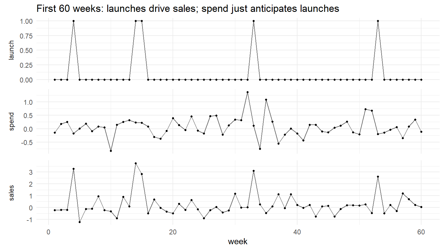
The chunk below simulates 200 weeks of exactly that system: a launch calendar drives both ad spend (via the marketing team’s advance knowledge of the calendar) and sales (via the launch itself). The true structural effect of spend on sales is zero. The first plot shows a 60-week slice of the raw series, so the confounding pattern becomes visible before we test anything.

set.seed(20260803)
library(ggplot2)
library(tidyr)

n <- 200

# the launch calendar is the true (unobserved) confounder
launch <- rbinom(n, size = 1, prob = 0.10)

# marketing books ad spend the week BEFORE a launch, having seen the calendar
# so spend[t] is elevated when launch[t+1] == 1
spend <- 0.5 * c(launch[-1], 0) + rnorm(n, sd = 0.3)

# only the launch itself drives sales; spend has zero structural effect
sales <- 3.0 * launch + rnorm(n, sd = 0.5)

df_plot <- data.frame(week = 1:60, launch = launch[1:60],
                      spend = spend[1:60], sales = sales[1:60]) |>
  pivot_longer(-week, names_to = "series", values_to = "value")
df_plot$series <- factor(df_plot$series, levels = c("launch", "spend", "sales"))

ggplot(df_plot, aes(week, value)) +
  geom_line(colour = "grey40") +
  geom_point(size = 0.9) +
  facet_wrap(~ series, ncol = 1, scales = "free_y", strip.position = "left") +
  labs(x = "week", y = NULL,
       title = "First 60 weeks: launches drive sales; spend just anticipates launches") +
  theme_minimal(base_size = 11) +
  theme(strip.placement = "outside", strip.background = element_blank(),
        panel.spacing = unit(0.6, "lines"))

Read the panels together. Each launch (top) is followed one week later by a sharp jump in sales (bottom). The middle panel shows that ad spend rises slightly in the week before each launch, because the marketing team is planning around the calendar. There is no causal channel from spend to sales in this data-generating process. But past spend still precedes the sales jump in time, and the launch calendar itself is invisible to any model that only looks at spend and sales. That is the entire mechanism the bivariate Granger test is about to fall for.

library(vars)
library(lmtest)

d   <- data.frame(spend = spend, sales = sales)
fit <- VAR(d, p = 2, type = "const")
gt  <- causality(fit, cause = "spend")$Granger

cat(sprintf("Granger test: does spend Granger-cause sales?\n"))

Granger test: does spend Granger-cause sales?

cat(sprintf("  F statistic:  %.2f\n", gt$statistic))

  F statistic:  12.69

cat(sprintf("  p-value:      %.4g\n", gt$p.value))

  p-value:      4.614e-06

cat(sprintf("  Reject H0 of no Granger causality at 5%%? %s\n",
            ifelse(gt$p.value < 0.05, "YES", "no")))

  Reject H0 of no Granger causality at 5%? YES

The test rejects the null of no Granger causality at any conventional level. It happily reports that spend Granger-causes sales, even though sales in this data-generating process are structurally unaffected by ad spend. The test is not broken. It is answering exactly the question it was built to answer, on data that were designed to hide the relevant confounder. A randomised experiment that fixed the launch calendar and varied spend independently would show a spend coefficient indistinguishable from zero. The two answers are not in conflict; they are answers to two different questions.

The general lesson is worth stating before turning the page. Forecasting tools are built and validated to answer “what will happen next,” using only the joint distribution as it has actually occurred, and they are evaluated by how small their out-of-sample prediction error is. Causal inference tools are built to answer “what would happen if I changed something,” which requires an additional assumption connecting the world you observed to the world you are asking about, whether that assumption is unconfoundedness, an instrument, a parallel-trends condition, or a structural model. Confusing the two is not a beginner’s mistake. It is an easy trap for a skilled analyst, precisely because the vocabulary crosses over: the word “causality” appears in both, the word “prediction” appears in both, and a test can be entirely correct on its own terms while being misapplied to a question it was never built to answer.

NoteA test can be right and still be misapplied

Granger causality is a legitimate and useful predictive diagnostic when used for what it is: forecasting model selection, VAR specification, and checking whether a candidate variable adds predictive value beyond a target’s own history. Modern extensions of the framework, including network Granger causality, non-linear and non-stationary variants, mixed-frequency versions, and Hawkes-process formulations for point-process data, remain active areas of methodological research (Shojaie and Fox, 2021). The failure is never in the test itself. The failure is in translating its result into the word “causes” without checking whether that word is doing the job the reader thinks it is.

Section II. Explain or predict? The distinction statistics almost forgot to make

The Granger trap is a specific instance of a much broader confusion, and it is worth pulling that broader confusion into focus before going any further. A team of marketing analysts and a team of causal econometricians can look at the same panel of ad-spend and sales data, build models that differ in almost every respect, and both walk away convinced their model is the right one. They are, without saying so, solving different problems. Shmueli (2010) diagnosed this confusion sharply in the statistics literature and stated the central claim that reorganises everything downstream: explanatory power and predictive power are neither necessary nor sufficient for each other. The same partition has since become standard in practitioner-oriented treatments of modern data analysis. Mahoney (n.d.), for instance, restates the distinction in compact form: prediction seeks a function \(\hat{f}\) that maps observed features \(X\) to an outcome \(Y\) with low error; estimation, or causal inference, seeks to uncover and quantify the underlying relationship, typically the parameters \(\beta\) in a model \(Y = g(X; \beta)\). Same \(X\), same \(Y\), different targets: the shape of \(\hat{f}\) on the one hand, the value of \(\beta\) on the other.

A model can have high explanatory power, meaning it correctly represents a hypothesized causal structure and its coefficients are theoretically interpretable, while having poor predictive power on new data. The reverse is equally possible: a model can predict new data very well while being causally uninterpretable, or even causally wrong. The intuition in each direction is easy to state. A correctly specified causal model estimated on a small, noisy sample can still generalize poorly out of sample, because being right about the mechanism does not compensate for having few observations of it. An atheoretical model stitched together from whatever correlations happen to predict well in a given dataset can forecast accurately for a long time without representing any mechanism at all.

Once the two goals are separated, the choices made at every stage of the modeling process separate with them. The comparison below tracks the five stages Shmueli (2010) works through in her paper, compressed into a form a practitioner can consult while scoping a project.

Stage	Explanatory / causal modeling	Predictive / forecasting modeling
Variable selection	Driven by a hypothesized causal structure (a DAG, a theory of confounding)	Driven by out-of-sample accuracy, regardless of interpretability
Model specification	Interpretable functional forms tied to theory	Algorithmic flexibility acceptable (gradient boosting, ensembles, neural nets)
What overfitting threatens	Validity of the estimated coefficient as a real relationship	Only the rule’s error rate, measured on held-out data
Validation	The identifying assumptions themselves	The rule’s error rate on data the model has not seen
What a “good” result is	A coefficient that is the correct, policy-relevant answer, however small	A forecast whose error is low, regardless of the mechanism behind it

The row worth unpacking, because it connects most directly to the identification vocabulary this blog has developed in its causal inference series, is validation. When a causal model is validated, what is being examined is not principally the model’s fit or its predictive error. What is being examined is whether the specific assumption that connects the observed data to the causal quantity of interest is credible in this application. Parallel trends in a difference-in-differences design is validated by looking at pre-treatment trajectories and by thinking hard about what else changed at the treatment date. Conditional independence in a matching design (Rosenbaum and Rubin, 1983) is validated by asking whether the covariates plausibly capture every channel through which selection into treatment operates. Predictive modeling has no analogue of this step, and it does not need one. The rule’s job is to forecast accurately on new data, and a held-out sample answers that question directly. This indifference to mechanism is not sloppiness. It is a correct response to a genuinely different objective, where the only thing that matters is the accuracy of the next prediction. Confusing the two forms of validation is one of the most common ways causal work goes wrong: a low cross-validated error is treated as evidence that the causal specification is correct, when the cross-validation exercise never examined the identifying assumption at all.

It is worth being direct about how easy this distinction is to lose in practice, particularly for a practitioner who is strong on one side of it. A causal inference background can create a very specific blind spot: the instinct to ask whether a specification is theoretically correct can lead someone to dismiss a model that would forecast very well, precisely because it lacks the interpretability that causal work correctly demands. I have done this myself on client work more than once, and I suspect most readers who have spent time in the causal inference literature will recognize the reflex. A forecasting background produces the symmetric blind spot: the instinct to trust whatever combination of features minimises cross-validated error can lead someone to over-interpret a predictive model’s coefficients as though they meant something causal, when the model was never built or validated for that purpose. A gradient-boosted model that forecast demand beautifully during a period of turbulence is not evidence that any of its top-ranked features actually caused demand to change. Neither blind spot is a failure of skill. Each is what happens when a well-trained instinct for one task is applied unchanged to the other.

The formal reason the two goals can diverge, even when using the exact same variables and the exact same data, sits in the decomposition of expected prediction error. Following Shmueli (2010) and Hastie, Tibshirani, and Friedman (2009), the expected squared prediction error at a point \(x\) decomposes as

\[ \text{EPE}(x) \;=\; E\!\left[(Y - \hat{f}(x))^2\right] \;=\; \sigma^2 \;+\; \bigl[E(\hat{f}(x)) - f(x)\bigr]^2 \;+\; \text{Var}(\hat{f}(x)), \]

that is, irreducible noise plus squared bias plus estimation variance. Minimising this quantity requires trading off bias and variance jointly. A predictive model is free to accept a biased estimate of any individual coefficient if that bias reduces the rule’s total out-of-sample error, because no individual coefficient is ever consulted on its own, only the rule’s output as a whole. A causal model does not have this freedom for the coefficient of interest. That specific coefficient is the object being reported and acted on, so an unbiased estimate of it is prioritised even at some cost to the model’s overall predictive accuracy.

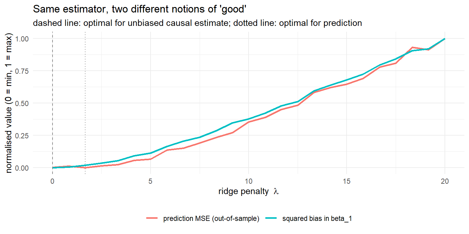
The chunk below makes the tension visible with the simplest possible example. Data are generated from a linear model with a target coefficient \(\beta_1 = 2\) and four nuisance coefficients. For a grid of ridge penalties \(\lambda\), we estimate the coefficients and compute two quantities: the squared bias in \(\hat\beta_1\) (relevant if the analyst wants to report or act on \(\beta_1\)) and the out-of-sample prediction mean squared error (relevant if the analyst just wants small forecast error). The two curves point to two different optimal choices of \(\lambda\).

set.seed(20260803)
library(ggplot2)

n <- 40; p <- 5; n_rep <- 400
lambdas    <- seq(0, 20, length.out = 25)
beta_true  <- c(2, rep(0.5, p - 1))

sim_at_lambda <- function(lam) {
  b1_hats <- numeric(n_rep); mses <- numeric(n_rep)
  for (i in 1:n_rep) {
    X  <- matrix(rnorm(n * p), n, p)
    y  <- X %*% beta_true + rnorm(n)
    b  <- solve(crossprod(X) + lam * diag(p), crossprod(X, y))
    b1_hats[i] <- b[1]
    X_te <- matrix(rnorm(200 * p), 200, p)
    y_te <- X_te %*% beta_true + rnorm(200)
    mses[i] <- mean((y_te - X_te %*% b)^2)
  }
  data.frame(lambda = lam,
             bias_sq  = (mean(b1_hats) - beta_true[1])^2,
             pred_mse = mean(mses))
}

res <- do.call(rbind, lapply(lambdas, sim_at_lambda))
res$bias_sq_norm  <- res$bias_sq  / max(res$bias_sq)
res$pred_mse_norm <- (res$pred_mse - min(res$pred_mse)) /
                    (max(res$pred_mse) - min(res$pred_mse))

ggplot(res) +
  geom_line(aes(lambda, pred_mse_norm, colour = "prediction MSE (out-of-sample)"),
            linewidth = 1) +
  geom_line(aes(lambda, bias_sq_norm, colour = "squared bias in beta_1"),
            linewidth = 1) +
  geom_vline(xintercept = 0, linetype = "dashed", colour = "grey50") +
  geom_vline(xintercept = res$lambda[which.min(res$pred_mse)],
             linetype = "dotted", colour = "grey50") +
  labs(x = expression(paste("ridge penalty  ", lambda)),
       y = "normalised value (0 = min, 1 = max)",
       colour = NULL,
       title = "Same estimator, two different notions of 'good'",
       subtitle = "dashed line: optimal for unbiased causal estimate; dotted line: optimal for prediction") +
  theme_minimal(base_size = 11) + theme(legend.position = "bottom")

The two curves tell the whole story of the section. If the analyst’s goal is to report an unbiased estimate of \(\beta_1\) (a causal parameter), the right choice is \(\lambda = 0\): any positive \(\lambda\) pulls \(\hat\beta_1\) toward zero and introduces bias. If the goal is to predict new observations with low error, \(\lambda = 0\) is strictly suboptimal: the prediction MSE curve reaches its minimum well inside the interior of the grid, at a \(\lambda\) where \(\hat\beta_1\) is provably biased. This is the mathematical seed of every operational difference in the table above. Shrinkage methods like ridge regression, which deliberately bias coefficients toward zero to reduce estimation variance, improve predictive accuracy for exactly this reason and would be unacceptable if the biased coefficient were itself the object of interest.

Framed this way, every identification strategy this blog has covered so far is doing, in Shmueli’s terms, exactly the validation work that explanatory modeling requires and predictive modeling does not. Parallel trends in a difference-in-differences design is a claim about counterfactuals, not about fit. Conditional independence in a matching or propensity score design (Rosenbaum and Rubin, 1983) is a claim about which pre-treatment variables must be adjusted for, not about which ones happen to improve out-of-sample accuracy. The exclusion restriction the reader will meet in the later instrumental variables post (Angrist, Imbens, and Rubin, 1996) is a claim about the channels through which the instrument can and cannot affect the outcome, not about the instrument’s predictive value for the treatment. None of these assumptions are checked by holding out a test set. They are checked by reasoning about the data-generating process, which is what makes them causal assumptions in the first place.

Knowing that the two jobs require different validation is necessary but not sufficient. The next section makes the distinction precise enough to state formally, using the language of interventions already familiar from earlier posts, so that “forecast” and “causal effect” stop being loosely related concepts and become two mathematically distinct objects.

TipThe one question that sorts it out

Before building any model, ask: if this model’s coefficients turned out to be wrong but its predictions stayed accurate, would that still count as a success? A yes points to predictive modeling, and the project should be scoped, validated and reported that way. A no points to explanatory modeling, and the identifying assumption is the deliverable. Most of the confusion I see on real projects comes from never asking the question at all.

Section III. Two questions, two counterfactuals

Two teams at a ride-hailing marketplace sit two desks apart, staring at the same warehouse of trip-level data. The forecasting team is preparing next week’s operational plan and needs to answer a straightforward question: how many rides will we complete next Sunday in Lisbon? Down the corridor, a pricing scientist is drafting a memo for the executive committee and must answer something that sounds similar but is not: what happens to completed rides if we raise driver incentives by ten percent next Sunday?

The same dataset feeds both analyses. The same SQL warehouse, the same dashboards, the same joins on the same trip IDs. Yet the two questions are objects of a fundamentally different nature. One asks about the future of the world as it is. The other asks about the future of a world that does not yet exist, a world we are proposing to create by pulling a lever. Everything that follows in this section is an attempt to make that distinction sharp enough to be mathematically useful.

The forecasting target

Forecasting seeks to characterise the conditional distribution of future observations given past information. In its most common form the target is the conditional expectation \(E[Y_{t+k} \mid X_t = x]\), the expected value of the outcome \(Y\) at time \(t+k\) given the features \(X_t\) observed at time \(t\). Where a point prediction is not enough, the target becomes the full predictive distribution \(P(Y_{t+k} \mid X_t = x)\), which describes the probability of each possible future outcome given the historical record.

In plain English, forecasting tries to learn what usually happens next given the patterns embedded in historical data. The critical property of these objects is that they live entirely inside the observed joint distribution of \((X, Y)\). No intervention is required to define them, and no counterfactual world is created to estimate them. If the process is stable enough for tomorrow to resemble yesterday, a well-tuned model of \(P(Y_{t+k} \mid X_t)\) will produce accurate ride forecasts. Nothing in this task requires a theory of why the data look the way they do.

The causal target

Now change the question. Management is no longer asking what will happen next Sunday if we do nothing different. They are asking what would happen if we raised driver incentives by ten percent. The estimand shifts entirely. Using the potential-outcomes framework, introduced in the statistical treatment-effect tradition by Neyman (1923) and Rubin (1974) and given its philosophical exposition in Holland (1986), we let \(Y(1)\) denote the outcome that would be observed under the intervention and \(Y(0)\) the outcome that would be observed without it. The average treatment effect is \(E[Y(1) - Y(0)]\), the expected difference between what would happen with the incentive change and what would happen without it, for the same population. Pearl (2009) writes the same idea using the do-operator, \(E[Y \mid do(X = x)]\), the expected outcome when we intervene to set \(X\) to \(x\), severing the mechanisms that would otherwise determine \(X\) from the historical data. Pearl’s distinction between seeing and doing is not decoration. The operation \(do(X = x)\) removes the arrows that ordinarily flow into \(X\) in the causal graph, so the resulting expectation is computed under a modified distribution that the observed data never directly sample. This is the same object the earlier post on counterfactuals on this blog developed in detail; here it is being reused to state the target of a decision, not to interpret a historical estimate.

The reader already knows the definitions. The point worth insisting on is the interpretation. \(Y(1)\) and \(Y(0)\) are not two observations. They are two states of the world, only one of which is ever realised for any given unit. The average treatment effect is a contrast between two distributions of outcomes that were never jointly observed and never can be. As Holland (1986) put it, this is the fundamental problem of causal inference: no unit is ever observed both treated and untreated at the same moment, so the estimand of interest lives in a distribution that was inferred rather than experienced.

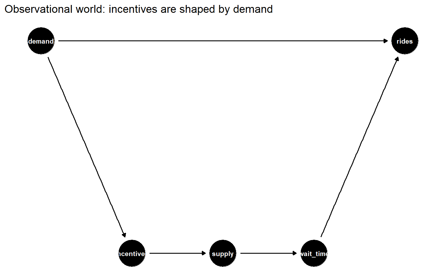
To make the do-operator less foreign, it helps to see it once as a picture. The chunk below draws the marketplace example: rider incentives affect supply, supply affects wait times, wait times affect completed rides, and rider incentives are themselves shaped by prior demand. The intervention \(do(\text{incentives} = x)\) severs the incoming edges into “incentives,” leaving the rest of the mechanism intact.

library(ggdag)
library(ggplot2)

dag_obs <- dagify(
  supply     ~ incentives,
  wait_time  ~ supply,
  rides      ~ wait_time + demand,
  incentives ~ demand,
  exposure   = "incentives",
  outcome    = "rides",
  coords = list(
    x = c(demand = 0, incentives = 1, supply = 2, wait_time = 3, rides = 4),
    y = c(demand = 1, incentives = 0, supply = 0, wait_time = 0, rides = 1)
  )
)

ggdag(dag_obs, text_size = 3) +
  theme_dag() +
  labs(title = "Observational world: incentives are shaped by demand")

Under \(do(\text{incentives} = x)\) the arrow from demand into incentives is removed. The forecasting task, computed from the observational graph on the left of that edge, silently absorbs the pathway demand -> incentives -> supply -> wait_time -> rides. The intervention question deliberately breaks it.

Why prediction does not identify intervention effects

This is where practitioners most often stumble. The temptation is to argue that if \(X\) predicts \(Y\) well enough, then acting on \(X\) should move \(Y\). Three examples make the fallacy obvious.

Rain predicts umbrella sales with startling accuracy. Nobody believes that stockpiling umbrellas will summon a storm. The arrow of causation runs from weather to consumer behaviour, and no intervention on umbrella supply changes the forecast for tomorrow’s rainfall.

Ice cream sales predict drownings across the summer months. Neither variable causes the other. Both respond to a common driver, temperature, together with the seasonality of outdoor activity. A model that used ice cream sales to allocate lifeguards would be well calibrated on historical data and dangerous in operational use.

In the marketplace itself, a spike in demand predicts a price increase in the next surge cycle. The predictive relationship is real. It is also useless as a policy lever, because nobody in operations would seriously argue that raising prices causes the demand that preceded it. The correlation reflects a dynamic pricing algorithm responding to demand shocks, not a causal effect running from price to quantity.

Predictive associations are features of the observed joint distribution \(P(X, Y)\). They can arise from \(X\) causing \(Y\), from \(Y\) causing \(X\), from a common cause affecting both, or from selection processes that involve no causal arrow between \(X\) and \(Y\) at all. Causal effects, by contrast, are features of a modified distribution, the distribution induced by intervention. The move from \(P(Y \mid X = x)\) to \(P(Y \mid do(X = x))\) is not a matter of estimator choice. It is a change of estimand.

Why interventions are difficult

The deeper reason the two targets diverge is that forecasting relies on the future resembling the past, and interventions deliberately break that assumption. Every serious business decision moves the data-generating process, not just the data.

In pricing, historical demand was recorded under a specific set of price points and competitive conditions. A predictive model trained on data around a €9.99 price point has no reliable evidence about what happens at €12.99, because consumer substitution, competitor response, and brand perception may all shift in ways the historical joint distribution never encoded.

In marketing, past advertising exposure is correlated with a long list of other factors that also drive sales, including the timing of promotions, the state of the funnel, and the composition of the audience reached. A predictive model captures the observed bundle. A causal question asks what happens to sales if we change advertising spending while everything else is held fixed, a state of affairs the observed data may never contain.

In product launches, the difficulty is starker. There is no historical data on a product that has not yet shipped. A predictive model cannot be fit at all. Any forecast of adoption or revenue requires reasoning about a new world, which is a causal exercise dressed up as prediction.

Marketplace incentives combine all three difficulties at once. Raising driver bonuses by ten percent shifts supply, changes surge dynamics, alters rider wait times, and feeds back into demand through the reliability channel. The moment we intervene, we are no longer asking about the world that generated our data. We are asking about a different world. Causal inference exists because we want to answer questions about that different world using data from this one.

The earlier posts in one line

The methods reviewed in the previous instalments of this series were all in the business of recovering causal quantities of the form \(E[Y \mid do(X = x)]\) or its conditional variants, not of minimising forecast error on a held-out sample. Difference-in-Differences leans on parallel trends. Matching leans on unconfoundedness given observed covariates. G-Computation leans on a correctly specified outcome model together with no unmeasured confounding. Synthetic Control leans on a convex combination of donor units that reproduces the pre-treatment trajectory. Their validation criteria are not out-of-sample predictive accuracy but the credibility of an identification assumption. The estimand was always causal; the machinery was designed accordingly.

Prediction versus intervention forecasting

Gische, West, and Voelkle (2021) draw exactly this line in the context of cross-lagged panel structural equation models. They distinguish between the prediction of future outcomes, formalised as \(E[Y_{t+k} \mid X_t = x]\), and the forecasting of causal effects of interventions, formalised as \(E[Y_{t+k} \mid do(X_t = x)]\). Their central observation is that these tasks are mathematically distinct even when performed on the same longitudinal dataset with the same variables and the same statistical model. Same data, same time indices, different estimands, different identification requirements, different answers. Their formal treatment is confined to cross-lagged panel structures with specific assumptions about time-invariant unobserved heterogeneity, so the result should not be over-generalised to all longitudinal data settings. Within that scope, their paper is the natural bridge between the causal inference series that preceded this post and the forecasting series that follows it, because it shows the two estimands, formalises the identification conditions for each, and refuses to let one masquerade as the other.

The consequences of that refusal are not academic. A forecast can be perfectly calibrated and still be entirely silent on, or actively misleading for, the decision the business is trying to make. The next section walks through exactly how that failure mode looks in practice.

Section IV. A forecast can be right and still be useless

Imagine a marketplace analytics team that has spent two years perfecting its weekly ride demand model. The forecast is accurate. Backtests are clean, holdout errors are small, and the model has beaten every alternative the team has thrown at it. Operations plans driver shifts around its numbers, finance uses it to project revenue, and supply planning treats it as ground truth. Everyone trusts the forecast, and rightly so.

Then, in a leadership meeting, the general manager asks a simple question: “What happens to demand if we raise driver incentives by ten percent next week?”

The room goes quiet, because the honest answer is that the forecasting model cannot say. It was never built to answer that question, and nothing about its predictive accuracy guarantees that it can. The model was trained to describe the future of the current system. The question is about the future of a modified system. Those are not the same object, and no amount of validation on historical data will bridge the gap between them.

Why accurate forecasts miss intervention questions

Forecasting models succeed because they exploit recurring patterns in historical data. Seasonality, trend, calendar effects, behavioural regularities, and cross-series dependencies are structural features of the observed process, and a good forecasting system learns to detect and extrapolate them. The core assumption, sometimes stated explicitly and often left implicit, is that future observations will emerge from the same data-generating process that produced past observations. Shmueli (2010) makes this point sharply in her discussion of predictive modeling: the goal is to minimise expected prediction error on new observations drawn from the same distribution, not to recover the underlying causal mechanism.

Interventions deliberately violate the stationarity assumption that makes forecasting work. The moment a manager changes prices, incentives, promotions, algorithms, product features, targeting rules, or matching logic, the organization is no longer asking about the world that generated the historical data. It is asking about a different world, one in which the very levers being pulled were held fixed, or moved through mechanisms different from the intended intervention, during the training period. The forecasting model has, by construction, no information about what happens when those levers move outside their historical range, or move in ways that were previously entangled with other factors the model has quietly absorbed.

Section III drew the formal line between \(E[Y \mid X = x]\) and \(E[Y \mid do(X = x)]\). In the panel data setting, Gische, West, and Voelkle (2021) show that these two quantities coincide only under specific identification conditions and in general differ, sometimes by a lot, sometimes with opposite signs. A forecasting model estimates the first quantity. A pricing decision requires the second.

The distinction is not academic. Schultz et al. (2024), working on demand forecasting for pricing at Zalando, show that a state-of-the-art transformer forecasting model performs well on-policy, when the pricing regime in the forecast horizon resembles the pricing regime in the training data, but degrades off-policy, when the forecast horizon contains price levels or discount patterns the model has not seen. Their causal architecture, which explicitly separates an outcome model, a treatment model, and an effect model along Double Machine Learning lines (Chernozhukov et al., 2018) using transformer components for each stage, “outperforms forecasting methods in off-policy settings while only slightly trailing in the on-policy setting,” in the paper’s own measured framing. The lesson generalises beyond their specific setting. Predictive accuracy earned in a stable pricing regime does not transfer to a regime that the pricing decision itself creates.

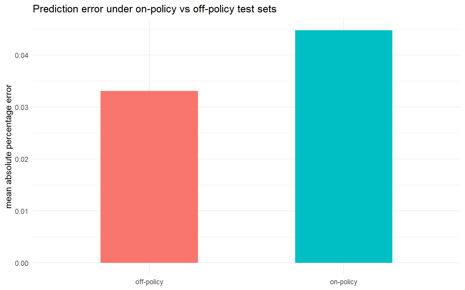
The pattern is easy to make visible with a stylised simulation. The chunk below generates weekly demand as a linear function of price plus noise, trains a naive forecasting model that treats price as just another covariate, and compares its performance under an on-policy holdout (prices drawn from the training range) against an off-policy holdout (prices shifted downward, as would occur under an aggressive promotional policy). The simulation is deliberately generous: the true relationship is linear, the covariate set is complete, and the model is correctly specified for the on-policy regime. In a real pricing application, where consumer substitution, competitor reaction, and inventory constraints all bend at the new price point, the off-policy gap is substantially larger than the one shown here.

set.seed(20260803)
library(ggplot2)

n_train <- 500
n_test  <- 200

# training data: price varies in a narrow historical range
price_train  <- rnorm(n_train, mean = 10, sd = 0.6)
demand_train <- 100 - 4 * price_train + rnorm(n_train, sd = 3)

# a naive predictive model just regresses demand on price
naive <- lm(demand_train ~ price_train)

# on-policy test set: prices drawn from the same range as training
price_on   <- rnorm(n_test, mean = 10, sd = 0.6)
demand_on  <- 100 - 4 * price_on + rnorm(n_test, sd = 3)
pred_on    <- predict(naive, newdata = data.frame(price_train = price_on))
mape_on    <- mean(abs(demand_on - pred_on) / demand_on)

# off-policy test set: prices shifted down by 20% (an aggressive discount policy)
price_off  <- rnorm(n_test, mean = 8, sd = 0.6)
demand_off <- 100 - 4 * price_off + rnorm(n_test, sd = 3)
pred_off   <- predict(naive, newdata = data.frame(price_train = price_off))
mape_off   <- mean(abs(demand_off - pred_off) / demand_off)

df <- data.frame(
  regime = c("on-policy", "off-policy"),
  MAPE   = c(mape_on, mape_off)
)
ggplot(df, aes(x = regime, y = MAPE, fill = regime)) +
  geom_col(width = 0.5, show.legend = FALSE) +
  labs(x = NULL, y = "mean absolute percentage error",
       title = "Prediction error under on-policy vs off-policy test sets") +
  theme_minimal()

Even under these best-case conditions, when the test set shifts to prices the model has never seen, the error rises. Any real deployment, where the pricing policy itself changes the composition of demand, would show a much larger gap. Predictive success and decision usefulness are not the same thing.

Effects of causes, causes of effects

Holland (1986) draws a distinction that has aged well and deserves more attention in applied work. Statistical questions, he argues, come in two flavours. Some ask about the effects of causes: given a well-defined intervention, what is its effect on an outcome of interest? Others ask about the causes of effects: given an observed outcome, what produced it? Holland is explicit that the potential outcomes framework, and by extension most of causal inference, is designed to answer the first kind of question, not the second. His slogan “no causation without manipulation” is the sharp end of a deeper claim: causal effects are defined by hypothetical interventions on things that could, in principle, be manipulated, and forecasting models rarely, if ever, satisfy that requirement by themselves.

Forecasting models sit in an even more restricted corner. They typically answer neither of Holland’s two questions. They identify useful predictors, variables whose values help reduce error in the conditional distribution of the outcome. A useful predictor is not the same thing as a cause, and it is certainly not the same thing as an intervention target.

The distinction is easier to see with concrete examples. In a marketplace, the number of active sessions in the last hour is often a strong predictor of the number of orders in the next hour. It would be a mistake to conclude that management should try to increase sessions in order to increase orders, since sessions and orders are jointly driven by a common set of factors, including demand shocks, marketing campaigns, weather, day-of-week patterns, and competitor behaviour. The predictive relationship is real and stable. The intervention on sessions, absent an intervention on those underlying drivers, may produce nothing at all.

In pricing, the average basket size is often a strong predictor of conversion. It does not follow that forcing customers into larger baskets will raise conversion, since basket size is itself an outcome of the same choice process that produces the conversion decision. In churn modeling, tenure is one of the most predictive features in any commercial dataset. It is also useless as an intervention target, since no product manager can move a customer’s tenure directly. In credit scoring, the number of recent credit inquiries predicts default. It is a poor policy instrument, because the inquiries are symptoms of the financial pressure that drives default rather than a cause of it.

The pattern is general. A variable can be strongly and stably associated with an outcome while being a poor intervention target. Forecasting rewards the first property. Decision-making requires the second.

Prediction, estimation, attribution

Efron (2020) offers a taxonomy that complements Holland’s and speaks directly to the modern practitioner. He distinguishes three tasks that statistical modeling can perform. Prediction assigns a value to a future outcome based on observed covariates. Estimation recovers a parameter of an underlying data-generating process, typically with an accompanying measure of uncertainty. Attribution assigns credit to specific predictors, asking which variables are doing the work. Efron’s Table 5 lays these differences out across six dimensions, contrasting the traditional “surface plus noise” regression model with the pure prediction algorithms that dominate modern machine learning, and noting that the two enterprises differ not only in method but in what they treat as scientific truth.

Efron’s central observation is that modern machine learning systems have become extraordinarily effective at prediction while providing very little in the way of estimation or attribution. Random forests, gradient boosting, deep neural networks, and their variants routinely achieve low prediction error on complex tasks. They typically achieve this by combining large numbers of weak learners in ways that make the underlying parameters difficult to interpret and the attribution of importance to specific features unstable. His prostate cancer illustration is striking: on a microarray dataset with roughly 6000 genes, a random forest predicts cancer status with only a handful of errors. Removing the single most important gene, then the top five, the top ten, the top twenty, and eventually the top several hundred features that the algorithm identifies as most important, and refitting on the remaining features, still yields essentially the same predictive performance. The information relevant to prediction is spread across the feature space in ways that resist the traditional notion of a small set of causal drivers.

None of this is a criticism of machine learning. It is a clarification of which question these systems are answering. A gradient boosting model that predicts next-week demand with low error is genuinely useful for capacity planning and staffing. It is not, without additional structure and additional assumptions, useful for evaluating what would happen if the pricing policy changed. The relevant assumptions are causal assumptions, and they cannot be extracted from the training data. Heckman (2008) makes the same point in the econometric tradition: causal parameters are defined by hypothetical manipulations of well-specified structural mechanisms, and no amount of pattern recognition in observational data will identify them without additional structure imported from theory or design. The econometric approach, in Heckman’s framing, is not opposed to prediction. It just refuses to conflate prediction with the answer to a policy question.

Goodhart’s law and the fragility of predictive relationships

There is a further reason to be cautious about turning a forecasting model into a decision engine. Predictive relationships tend to be stable as long as the organization is watching them. They tend to degrade the moment the organization starts optimising against them.

The pattern is old enough to have a name. Goodhart’s law, in the formulation popularised by Strathern (1997), states that when a measure becomes a target, it ceases to be a good measure. The mechanism behind it is precisely the mechanism this section has been describing. A predictive relationship is a statement about the joint distribution of variables in a particular environment, produced by a particular set of behaviours and mechanisms. When decision-makers begin to act on the relationship, they change those behaviours and mechanisms, and the relationship shifts.

The empirical literature is full of examples. Credit models built on historical repayment data lose predictive power once lenders start using them to set terms, because the pool of borrowers who accept the terms changes in response. Recommendation systems trained on historical click data drift once they start driving what users see, because the future click distribution is shaped by the recommender itself. Pricing models trained on observational data are notoriously unreliable off-policy, because the price variation in the training data was generated by a pricing policy that the new policy is designed to replace.

The general moral is that observing a pattern and acting on a pattern are different activities. Observation leaves the pattern intact. Action, especially systematic action at scale, tends to erode it. A model that has proven itself as a forecaster in a stable environment has proven nothing about its behaviour in an environment where it is being used to make decisions.

Why organizations experiment

The natural response to all of this, and the one that mature product and pricing organizations converge on, is experimentation. Randomized controlled trials, A/B tests, holdout experiments, switchback designs, geo experiments, and the various instruments in the modern causal toolkit exist for a specific reason: they generate variation in the treatment that is independent, by construction, of the factors that ordinarily determine it. That independence is what makes the resulting estimate an estimate of a causal effect rather than of a conditional expectation. In the language of the previous sections, the experiment engineers the equality between \(E[Y \mid do(X = x)]\) and \(E[Y \mid X = x]\) that observational data cannot deliver on its own.

Organizations do not run experiments because their forecasting is inadequate. Marketplace teams with excellent demand forecasts still run pricing experiments. Growth teams with excellent conversion models still run onboarding experiments. Product teams with excellent engagement forecasts still run feature experiments. They do so because the questions that matter to them, questions about the effect of changing something, are not questions that any forecasting model can answer on its own.

Once an organization internalises that predictive accuracy does not answer intervention questions, the investment in experimentation infrastructure begins to look less like a cost centre and more like the only reliable way to answer policy questions. Yet even with a clean experimental estimate in hand, the analyst is not done. The next section examines what forecasting and causal inference share, once we look past the vocabulary: the common problem of reasoning about quantities the data do not directly reveal.

Section V. Different questions, similar challenges

After four sections spent sharpening the distinction between forecasting and causal inference, it may feel strange to open this one by softening it. The distinction is real, and nothing that follows retracts it. But once we look past the vocabulary, both disciplines confront a common obstacle: they must reason about quantities that lie outside the data at hand. The forecaster does not observe the future. The causal analyst does not observe the counterfactual. Both are, in a very literal sense, filling in missing data. This is the argument advanced, in its most explicit form, by Fernández-Loría (2025), who frames causal inference as a structured instance of prediction under distribution shift. The claim is not that the two questions are the same. The claim is that the machinery required to answer either question must, at some point, cross the same bridge, the bridge of generalisation.

The purpose of this section is to make that bridge visible without dissolving the distinction we have worked to establish.

Generalisation as the common challenge

Forecasting assumes that the relationships learned from historical data will continue to hold in the deployment environment. Causal inference assumes that the outcomes observed under one treatment condition can be used to recover the outcomes that would have been observed under another. Both assumptions are, in their own way, assumptions about generalisation: from the observed to the unobserved, from the sampled to the target, from what was to what would have been.

Fernández-Loría (2025) makes this parallel precise. In predictive modeling, the source domain is a labeled dataset and the target domain is a set of cases where the label is unknown. In causal inference, the source domain is the set of treated units observed under treatment (and control units observed under control), and the target domain is the set of counterfactual outcomes that were never realised. In both cases, the analyst holds outcomes drawn from one distribution and wants to say something credible about outcomes drawn from another. In both cases, the data alone do not settle the question. Something else must, whether assumptions, structure, domain knowledge, or design.

The issue, then, is not whether the missing quantity is future or counterfactual. The issue is whether the assumptions that justify the leap from what we see to what we want are credible in the specific setting we are working in.

Distribution shift and selection bias play analogous roles

The two disciplines have inherited different vocabularies for the ways in which generalisation can fail. Forecasting worries about distribution shift: the joint distribution of features and outcome in training differs from the joint distribution at deployment. Prices move, competitors enter, user behaviour evolves, seasonality bends. A model trained on stationary history walks into a non-stationary future and misfires.

Causal inference worries about selection bias: treated and untreated units differ systematically in ways that distort the comparison. High-value customers self-select into premium tiers. Sophisticated advertisers opt into new bidding features. Healthier patients receive elective treatments. A naive difference in means reflects both the treatment effect and the difference between the groups.

These are not the same problem. Distribution shift arises from temporal or environmental change; selection bias, from non-random assignment. They require different remedies. But they are structurally analogous. Both describe situations in which the distribution generating the observed data differs from the distribution the analyst actually cares about. Both require assumptions, whether stationarity, unconfoundedness, overlap, or ignorability, that cannot be tested from the data alone. Neither discipline gets to escape the question of whether generalisation is warranted.

External validity is a forecasting problem in disguise

Suppose a pricing team runs a clean experiment in one market and estimates a price elasticity with tight confidence intervals. Identification is unimpeachable, the design is randomised, the estimand is well-defined. Now the team is asked to use that elasticity to set prices in a different market, or in the next quarter, or on a different segment of users. Suddenly the causal estimate, however well identified, is being forecast into an environment where it was not measured.

Heckman (2008) has been particularly forceful on this point. In his paper on econometric causality he lays out three policy-evaluation problems that are routinely conflated. Problem P1 is identifying a causal parameter in the environment where it was estimated, the classical internal-validity task. Problem P2 is transporting that parameter to a different environment, the external-validity task. Problem P3 is forecasting the impact of a policy that has never been implemented at all, at any scale, on any population. Serious applied work rarely stops at P1. Almost every business question of interest involves P2 or P3, and the honest analyst has to notice which one is on the table. Gische, West, and Voelkle (2021) make a related point at the level of individual heterogeneity: the treatment level that is optimal for the average unit can be strictly suboptimal for a specific unit whose covariates differ from the mean. The same logic applies at the level of markets, segments, and time periods. An identified causal effect is a statement about a specific population under specific conditions; whether it remains useful in a new one is a separate question, and it is a question that involves forecasting.

The pattern is everywhere in practice. An A/B test conducted on high-frequency users. A price elasticity estimated during a promotional window. A marketplace intervention tested in one city and scaled to twenty. An experiment on desktop generalised to mobile. In each case, the identification problem is solved. The transportability problem is not.

When prediction machinery meets causal ends

The clearest evidence that the two disciplines share a common problem is that some of the most useful modern causal methods are borrowed straight from the forecasting toolkit. Athey et al. (2021) develop matrix completion methods for causal panel data, imputing the untreated counterfactual outcomes for treated units by treating the panel of control outcomes as a low-rank matrix with missing entries, exactly the machinery used in recommender systems. The estimand is causal; the machinery is predictive. Goldin, Nyarko, and Young (2024) push the same idea further with SyNBEATS, a neural-network forecaster for synthetic-control-style causal panel problems, and show that off-the-shelf forecasting architectures can compete with dedicated causal estimators on impact evaluation tasks. Neither paper claims that prediction and causal inference are the same task. Both demonstrate that the assumptions justifying generalisation, once made explicit, allow prediction machinery to serve causal ends.

Fernández-Loría’s reframing

Fernández-Loría (2025) pushes the argument one step further. If causal inference is, at its core, the task of predicting outcomes we have not observed under conditions we have not sampled, then perhaps it should be understood as a special case of prediction under distribution shift, where the shift is generated by treatment assignment rather than by time or geography. The paper is careful to preserve the specificity of the causal problem: it explicitly states that causal inference “is special, a special case of prediction,” and that the counterfactual framing, the potential outcomes, the causal diagrams, and the identification strategies are essential rather than optional. The reframing is not that causal inference dissolves into prediction, but that both rest on the same underlying leap and can benefit from each other’s tools.

One does not have to fully endorse this reframing to find it useful. Even readers who prefer to keep causal inference on its own methodological footing, because the counterfactual object is genuinely distinct and Pearl’s (2009) structural framework treats it as such, can accept the narrower observation: both forecasting and causal inference must, at some point, defend the credibility of a generalisation the data cannot verify. The mathematical languages differ. The philosophical anxieties do not.

Where this leaves the decision

Most real business decisions therefore require not one act of generalisation but two. First, from observed outcomes to an estimated causal effect, the identification problem. Second, from the estimated causal effect to the environment in which the decision will actually be implemented, the transportability problem. The two problems interact. An effect that is perfectly identified but poorly transportable is a decision that will look confident on the slide and disappointing in the deployment. An effect that is transportable in principle but poorly identified from the available data is a decision built on sand. Forecasting and causal inference each own one half of that chain; neither owns the whole.

The version of this task that pricing teams, marketplace teams, and revenue management teams actually face is a third question, distinct from either forecasting or causal inference in isolation: what will happen, in the future, if a particular policy is implemented? This is the question that combines the two: it requires a credible causal effect and a credible forecast of the environment in which that effect will operate. Recent work on causal forecasting for pricing (Schultz et al., 2024) shows how demanding the joint requirement is, and how the same dataset can support very different conclusions depending on whether the analyst treats the price variable as a covariate or as a treatment.

Sophisticated product, pricing, and marketplace organizations rarely choose between prediction and causal inference for exactly this reason. They use both, deliberately and in sequence. They forecast demand to plan capacity and set expectations. They estimate elasticities to price rationally against those forecasts. They run experiments to validate the elasticities and to detect drift when it occurs. They build decision systems that consume both the forecasts and the causal estimates. They update the forecasts as the world moves. They re-estimate the effects as new experiments accumulate. And they repeat this cycle continuously, because the environment never stops moving. In this architecture, forecasting and causal inference are not competing; they are complementary inputs into a single decision loop. The forecast tells the organization what to expect. The causal estimate tells it how its actions will change what to expect. Neither is sufficient. Both, together, are close to sufficient for the kinds of decisions revenue management, pricing science, and marketplace science routinely have to make. Teams that forecast without estimating elasticities eventually find themselves unable to explain why their forecasts miss when policy changes. Teams that estimate elasticities without forecasting eventually find themselves unable to translate those estimates into next-quarter decisions. The complementarity is not optional. It is structural.

Conclusion. The question comes first

Most debates in analytics begin with models: machine learning versus econometrics, prediction versus explanation, experiments versus observational methods, interpretable models versus black boxes, regularised regression versus deep neural networks. These debates generate strong opinions and occasionally useful methodological progress. They also almost always begin too late.

The most consequential decision in any quantitative analysis occurs before methodology enters the picture. It occurs when the analyst chooses, explicitly or by default, which question the analysis is meant to answer. Different questions produce different estimands; different estimands require different tools, different assumptions, and different data. Method selection is downstream of question selection, and no amount of algorithmic sophistication rescues an analysis that has silently answered the wrong question. Stated without ornament: the question defines the estimand, the estimand defines the method, and the method defines the interpretation. Reversing that order is the single most common source of error in applied work.

The data do not tell you which question you are answering. The same dataset, analysed with the same software, by the same analyst, can yield radically different quantities depending on whether the target is a forecast, a causal effect, or a policy simulation. Only the analyst can decide which one is on the table. That is why a perfectly executed analysis of the wrong estimand is worse than an approximate analysis of the right one: the first produces confidence without content, while the second at least points in a useful direction. This is not a counsel of humility. It is a counsel of precision.

The article began with Granger. His 1969 framing of predictive causality was defined explicitly in terms of forecast improvement, not intervention effects, and treating it as if it settled questions about the consequences of manipulation has generated decades of confusion in fields far beyond econometrics. Forecasting is not causal inference. Causal inference is not forecasting. But both become more powerful when practitioners understand exactly which question they are trying to answer, and both become dangerous when practitioners use the machinery of one to answer questions belonging to the other. The strongest analysts, in my experience, are not those who know the most sophisticated methods. They are those who identify the correct question before choosing a method, the ones who pause, before opening the notebook, to ask what quantity would actually inform the decision at hand. That pause is the entire discipline. The estimand comes first. The estimator comes second. Everything else comes after.

References

Angrist, J. D., Imbens, G. W., & Rubin, D. B. (1996). Identification of causal effects using instrumental variables. Journal of the American Statistical Association, 91(434), 444–455.

Athey, S., Bayati, M., Doudchenko, N., Imbens, G., & Khosravi, K. (2021). Matrix completion methods for causal panel data models. Journal of the American Statistical Association, 116(536), 1716–1730.

Chernozhukov, V., Chetverikov, D., Demirer, M., Duflo, E., Hansen, C., Newey, W., & Robins, J. (2018). Double/debiased machine learning for treatment and structural parameters. The Econometrics Journal, 21(1), C1–C68.

Efron, B. (2020). Prediction, estimation, and attribution. Journal of the American Statistical Association, 115(530), 636–655.

Fernández-Loría, C. (2025). Causal inference isn’t special: Why it’s just another prediction problem. arXiv preprint arXiv:2504.04320.

Gische, C., West, S. G., & Voelkle, M. C. (2021). Forecasting causal effects of interventions versus predicting future outcomes. Structural Equation Modeling: A Multidisciplinary Journal, 28(3), 475–492.

Goldin, J., Nyarko, J., & Young, J. (2024). Forecasting algorithms for causal inference with panel data. arXiv preprint arXiv:2208.03489.

Granger, C. W. J. (1969). Investigating causal relations by econometric models and cross-spectral methods. Econometrica, 37(3), 424–438.

Hastie, T., Tibshirani, R., & Friedman, J. (2009). The Elements of Statistical Learning: Data Mining, Inference, and Prediction (2nd ed.). Springer.

Heckman, J. J. (2008). Econometric causality. International Statistical Review, 76(1), 1–27.

Holland, P. W. (1986). Statistics and causal inference. Journal of the American Statistical Association, 81(396), 945–960.

Imbens, G. W., & Rubin, D. B. (2015). Causal Inference for Statistics, Social, and Biomedical Sciences: An Introduction. Cambridge University Press.

Mahoney, M. (n.d.). Prediction and estimation. In Modern Data Analysis [online book]. Retrieved from https://mike-data-analysis.share.connect.posit.cloud/prediction-and-estimation.html

Neyman, J. (1923). On the application of probability theory to agricultural experiments. Essay on principles. Section 9. Translated in Statistical Science, 5(4), 465–472 (1990).

Pearl, J. (2009). Causality: Models, Reasoning, and Inference (2nd ed.). Cambridge University Press.

Rosenbaum, P. R., & Rubin, D. B. (1983). The central role of the propensity score in observational studies for causal effects. Biometrika, 70(1), 41–55.

Rubin, D. B. (1974). Estimating causal effects of treatments in randomized and nonrandomized studies. Journal of Educational Psychology, 66(5), 688–701.

Schultz, D., Stephan, J., Sieber, J., Yeh, T., Kunz, M., Doupe, P., & Januschowski, T. (2024). Causal forecasting for pricing. arXiv preprint arXiv:2312.15282.

Shmueli, G. (2010). To explain or to predict? Statistical Science, 25(3), 289–310.

Shojaie, A., & Fox, E. B. (2021). Granger causality: A review and recent advances. arXiv preprint arXiv:2105.02675.

Strathern, M. (1997). “Improving ratings”: Audit in the British university system. European Review, 5(3), 305–321.