---
title: "The Causal Compass: From Classical DiD to the Callaway–Sant'Anna Framework"
description: "Why staggered rollout analyses using TWFE can be misleading, and how to fix it. A practitioner's guide from the canonical 2×2 DiD to cohort-time ATTs, with full R implementation."
date: 2026-06-08
categories: [causal inference, econometrics, difference-in-differences, R]
#draft: true
---
```{r setup, include=FALSE}
knitr::opts_chunk$set(
echo = TRUE,
message = FALSE,
warning = FALSE,
fig.align = "center",
out.width = "100%"
)
```
## The CEO's Dilemma: Was It Really You?
Your company just completed a phased rollout of a new pricing algorithm. Deployed to the Northeast in Q1, the Midwest in Q2, and the South in Q3. Internal analytics reports a **4.8% improvement in gross margin**. The board is pleased. The CFO wants to accelerate the next initiative.
Before you sign the budget: **did your algorithm cause that improvement?**
Your VP of Data ran the standard two-way fixed effects regression. The coefficient is 4.8%, p-value < 0.01. Looks solid. But here is the uncomfortable truth that even many sophisticated analytics teams do not know: in a staggered rollout design like this one, that regression may not be estimating a policy-relevant average treatment effect. It is estimating a non-transparent weighted average of pairwise comparisons, driven by group sizes, treatment timing variance, and residual variation in treatment, some of which are economically nonsensical, some of which receive negative weights, and none of which corresponds to any question a rational business leader would want answered.
This is not a hypothetical risk. Goodman-Bacon (2021) demonstrated that TWFE estimates in staggered settings can be negative even when the true treatment effect is positive for every treated unit at every time period. This sign reversal occurs because already-treated units serve as implicit controls for later-treated units, and their treatment effects contaminate the comparison. The resulting bias can be large enough to reverse the sign, leading to materially incorrect strategic decisions, such as scaling back programmes that are working or expanding those that are not.
This article gives you the tools to get it right.
By the end you will understand:
1. How classical DiD works and exactly when it stops working
2. Why TWFE can fail under staggered adoption: the Goodman-Bacon decomposition in plain language
3. How Callaway and Sant'Anna (2021) builds valid causal estimates from first principles
4. The full menu of ATT aggregations and what business question each one answers
5. A complete R implementation using real minimum-wage data from the `did` package
---
## Part I: Classical Difference-in-Differences {#part-i}
### The Counterfactual Problem
Every causal question has the same structure: compare what *did* happen to what *would have happened* without the intervention. We observe the former but can never directly observe the latter. That unobserved alternative is the **counterfactual**, the fundamental object of causal inference.
The entire DiD toolkit is an answer to one question: *where do we find a credible proxy for the missing counterfactual?*
DiD's answer is elegant: use a **control group's change over time** as an estimate of the counterfactual change for the treated group.
### The 2×2 Setup
The canonical DiD design has four cells: two groups (treated, control) and two time periods (pre, post). The parameter of interest is the **average treatment effect on the treated** (ATT), and the estimator is:
$$\widehat{ATT} = \underbrace{(\bar{Y}^{T}_{post} - \bar{Y}^{T}_{pre})}_{\text{Change for treated}} - \underbrace{(\bar{Y}^{C}_{post} - \bar{Y}^{C}_{pre})}_{\text{Change for control}}$$
The first difference captures the total change for treated units. The second difference subtracts the change that would have occurred anyway due to common time trends. Together they isolate the treatment effect. Note that the ATT is the effect for the treated group specifically; it differs from the ATE (average treatment effect on the entire population) unless treatment is randomly assigned.
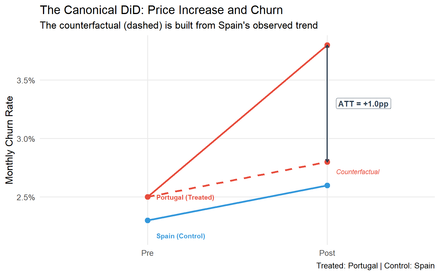
**A concrete business example.** You raise prices in Portugal but not in Spain. You want the causal impact on monthly churn:
| Group | Pre-Increase | Post-Increase | Change |
|:------|:------------:|:--------------:|:------:|
| Portugal (Treated) | 2.5% | 3.8% | +1.3pp |
| Spain (Control) | 2.3% | 2.6% | +0.3pp |
| **DiD Estimate (ATT)** | | | **+1.0pp** |
The price increase *caused* an estimated 1.0 percentage-point rise in churn, after netting out the common macro trend affecting both markets. This is the ATT: the average effect on the market that actually received the treatment.
```{r canonical-did, fig.cap="The canonical 2×2 DiD. Portugal's counterfactual (dashed) is constructed from Spain's trend. The ATT is the gap between observed and counterfactual outcomes after treatment."}
library(ggplot2)
library(dplyr)
library(tidyr)

# Canonical DiD data
did_data <- tibble(
  period = c("Pre", "Pre", "Post", "Post"),
  group  = c("Portugal (Treated)", "Spain (Control)",
             "Portugal (Treated)", "Spain (Control)"),
  churn  = c(2.5, 2.3, 3.8, 2.6)
)

# Counterfactual: Portugal following Spain's trend
cf <- tibble(
  period = c("Pre", "Post"),
  group  = c("Portugal (Counterfactual)", "Portugal (Counterfactual)"),
  churn  = c(2.5, 2.5 + (2.6 - 2.3))  # Portugal pre + Spain's change
)

plot_data <- bind_rows(did_data, cf) %>%
  mutate(
    period = factor(period, levels = c("Pre", "Post")),
    ltype  = ifelse(group == "Portugal (Counterfactual)", "dashed", "solid"),
    colour = case_when(
      group == "Portugal (Treated)"      ~ "#E74C3C",
      group == "Spain (Control)"         ~ "#3498DB",
      group == "Portugal (Counterfactual)" ~ "#E74C3C"
    )
  )

ggplot(plot_data, aes(x = period, y = churn, group = group,
                      colour = colour, linetype = ltype)) +
  geom_line(linewidth = 1.2) +
  geom_point(size = 3) +
  annotate("segment",
           x = 2, xend = 2,
           y = cf$churn[2], yend = 3.8,
           arrow = arrow(ends = "both", length = unit(0.15, "cm")),
           colour = "#2C3E50", linewidth = 0.8, linetype = "solid") +
  annotate("label", x = 2.05, y = (3.8 + cf$churn[2]) / 2,
           label = "ATT = +1.0pp", hjust = 0,
           colour = "#2C3E50", size = 3.5, fontface = "bold") +
  scale_colour_identity() +
  scale_linetype_identity() +
  scale_y_continuous(labels = scales::label_number(suffix = "%")) +
  labs(
    title    = "The Canonical DiD: Price Increase and Churn",
    subtitle = "The counterfactual (dashed) is built from Spain's observed trend",
    x = NULL, y = "Monthly Churn Rate",
    caption  = "Treated: Portugal | Control: Spain"
  ) +
  annotate("text", x = 1.05, y = 2.5,
           label = "Portugal (Treated)", colour = "#E74C3C",
           fontface = "bold", hjust = 0, size = 3) +
  annotate("text", x = 1.05, y = 2.17,
           label = "Spain (Control)", colour = "#3498DB",
           fontface = "bold", hjust = 0, size = 3) +
  annotate("text", x = 2.05, y = 2.72,
           label = "Counterfactual", colour = "#E74C3C",
           hjust = 0, size = 3, fontface = "italic") +
  theme_minimal(base_size = 13) +
  theme(legend.position = "none",
        panel.grid.minor = element_blank())
```
### The Parallel Trends Assumption
The DiD estimate is only valid under one critical assumption:
> **Parallel Trends**: In the absence of treatment, the average outcomes for treated and control groups would have followed the same trajectory over time.
Formally, denoting $Y_t(0)$ as the untreated potential outcome:
$$\mathbb{E}[Y_t(0) - Y_{t-1}(0) \mid D = 1] = \mathbb{E}[Y_t(0) - Y_{t-1}(0) \mid D = 0]$$
This assumption is untestable in the post-treatment period: we never observe $Y_t(0)$ for treated units after treatment. What we *can* do is inspect pre-treatment trends as supporting evidence. If the groups were on parallel paths before treatment, it is more credible (though not certain) that they would have remained so.
::: {.callout-important}
**The Parallel Trends assumption does not require the groups to have the same outcome *levels*, only the same *trend*.**
It is a statement about what would have happened in a counterfactual world, not about what we actually observe.
:::
### Estimation via TWFE: Why It Works in 2×2
In the canonical setting, the DiD estimate is identical to the coefficient $\hat{\beta}^{TWFE}$ from this regression:
$$Y_{it} = \alpha_i + \lambda_t + \beta^{TWFE} D_{it} + \varepsilon_{it}$$
where $\alpha_i$ are unit fixed effects, $\lambda_t$ are time fixed effects, and $D_{it} \in \{0,1\}$ is the treatment indicator (equal to 1 when unit $i$ is treated at time $t$, 0 otherwise). The unit FEs absorb time-invariant group differences; the time FEs absorb common shocks; $\beta^{TWFE}$ captures the residual, which is exactly the DiD estimate.
In a 2×2 design, TWFE is equivalent to DiD. This is the source of its appeal, and the source of a dangerous false confidence when applied to more complex settings.
---
## Part II: The Staggered Adoption Problem {#part-ii}
### What Is Staggered Adoption?
Real business rollouts rarely follow the tidy 2×2 pattern. The following are representative examples:
| Business Context | Staggered Pattern |
|:----------------|:-----------------|
| Software feature rollout | Wave 1: Premium customers (Jan); Wave 2: Mid-market (Apr); Wave 3: SMB (Jul) |
| New store format | Pilot: 20 stores (2022); Expansion: 80 stores (2023); Full: 200 stores (2024) |
| Minimum wage increase | States adopt at different years (2015 through 2022) |
| Marketing automation | Deployed by region as infrastructure is ready |
| Pricing algorithm | Rolled out market-by-market over 12 months |
This is **staggered treatment adoption**: different units (regions, stores, customers, states) receive treatment at different calendar times. For decades, the standard practice was simply to run TWFE on the full panel and interpret the coefficient as the average treatment effect. That coefficient can be misleading when treatment effects vary across cohorts or over time.
### The Goodman-Bacon Decomposition Theorem
Goodman-Bacon (2021) delivered the definitive diagnosis. He proved that in a staggered design, the TWFE estimator is a variance-weighted average of all possible 2×2 DiD comparisons that can be formed from the data.
With $K$ timing cohorts, this produces $O(K^2)$ pairwise comparisons. Some are economically valid. Others are contaminated.
```{mermaid}
%%{init: {'theme':'base','themeVariables':{'primaryColor':'#EBF5FB','edgeLabelBackground':'#fff','fontSize':'14px'}}}%%
flowchart TD
    A["TWFE coefficient β̂"] --> B["Variance-weighted average of all<br/> pairwise 2×2 DiDs"]
    B --> C["Type 1 <br/> Early-treated vs Never-treated<br/>✅ Clean"]
    B --> D["Type 2 <br/> Late-treated vs Never-treated<br/>✅ Clean"]
    B --> E["Type 3 <br/> Late-treated vs Early-treated<br/>❌ Contaminated"]
    C --> F["Valid comparison<br/>Receives positive weight under standard decomposition"]
    D --> G["Valid comparison<br/>Receives positive weight under standard decomposition"]
    E --> H["Already-treated units used as controls <br/> Outcomes contaminated by their own treatment effect <br/> Weights can be negative (non-convex averaging)"]

    style E fill:#FADBD8,stroke:#E74C3C
    style H fill:#FADBD8,stroke:#E74C3C
    style C fill:#D5F5E3,stroke:#27AE60
    style D fill:#D5F5E3,stroke:#27AE60
    style F fill:#D5F5E3,stroke:#27AE60
    style G fill:#D5F5E3,stroke:#27AE60
```
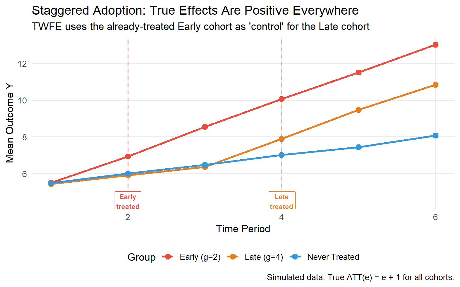
**The contaminated comparison.** Suppose Cohort A is treated at $t=2$ and Cohort B is treated at $t=4$. TWFE forms a comparison where Cohort B is the "treated" unit and Cohort A (already treated) serves as the "control" during periods 3 and 4. But Cohort A's outcomes in those periods include Cohort A's own treatment effect. If treatment effects vary across cohorts or over time, this comparison is contaminated and its contribution to the TWFE estimate can receive negative weight.
### The Negative Weights Problem: A Numerical Example
Let us make this concrete. Imagine three cohorts:
- **Cohort E** (Early): treated at $t=2$, with treatment effects that grow over time (ATT = 1 at $t=2$, 3 at $t=3$, 5 at $t=4$, 7 at $t=5$)
- **Cohort L** (Late): treated at $t=4$, with ATT = 1 at $t=4$, 3 at $t=5$
- **Cohort N**: never treated
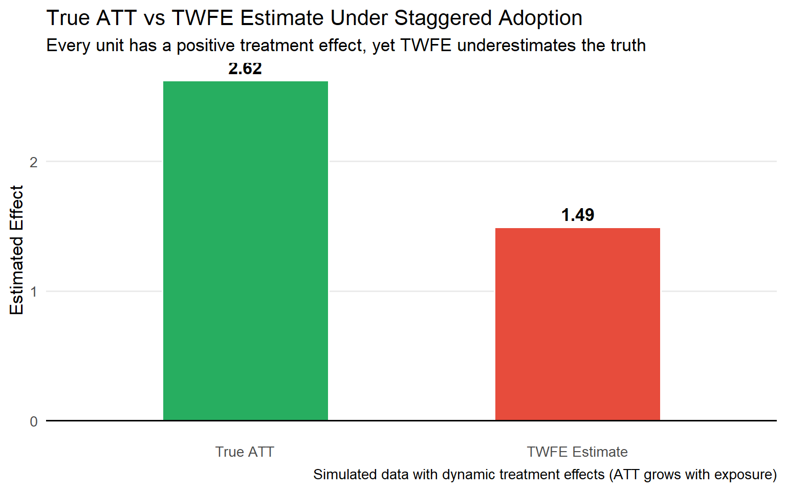
Every true treatment effect is positive. But the Goodman-Bacon decomposition reveals two distinct problems in this setting. First, TWFE forms a Late-vs-Early comparison that uses Cohort E's outcomes (already contaminated by its own treatment effect) as the counterfactual for Cohort L, a substantively invalid comparison. Second, because Cohort E's treatment effects grow over time (it has been treated longer), this contaminated comparison can receive negative weight in the variance-weighted TWFE average. Depending on group sizes and timing, the overall TWFE coefficient can be biased downward or even negative.
```{r negative-weights-sim, fig.cap="Simulated staggered adoption: every true ATT is positive, yet TWFE produces a downward-biased estimate in this configuration due to the contaminated comparison between early-treated (used as control) and late-treated cohorts. The direction and magnitude of bias depend on group sizes, timing, and the specific pattern of effect heterogeneity."}
library(dplyr)
library(ggplot2)
library(tidyr)

set.seed(42)
n_per_group <- 100
periods     <- 1:6

# Draw unit fixed effects at the unit level first, then expand
n_units <- 3 * n_per_group
unit_ids <- 1:n_units
unit_fes <- rnorm(n_units, sd = 1)

# True ATTs grow with exposure: ATT(e) = e + 1
sim_df <- expand.grid(id = unit_ids, t = periods) %>%
  as_tibble() %>%
  arrange(id, t) %>%
  mutate(
    group = case_when(
      id <= n_per_group               ~ "Early (g=2)",
      id <= 2 * n_per_group           ~ "Late (g=4)",
      TRUE                            ~ "Never Treated"
    ),
    first_treat = case_when(
      group == "Early (g=2)"  ~ 2,
      group == "Late (g=4)"   ~ 4,
      TRUE                    ~ Inf
    ),
    # Unit FE: same value for all time periods of the same unit
    unit_fe     = unit_fes[id],
    Y0          = 5 + unit_fe + 0.5 * t + rnorm(n(), sd = 0.5),
    # Treated potential outcome: ATT = e + 1 (e = event time, exposure duration)
    e           = ifelse(is.finite(first_treat), t - first_treat, -Inf),
    Y1          = Y0 + ifelse(e >= 0, e + 1, 0),
    D           = as.integer(t >= first_treat & is.finite(first_treat)),
    Y           = ifelse(D == 1, Y1, Y0)
  )

# Compute group means
means_df <- sim_df %>%
  group_by(group, t) %>%
  summarise(Y_mean = mean(Y), .groups = "drop")

ggplot(means_df, aes(x = t, y = Y_mean, colour = group, group = group)) +
  geom_vline(xintercept = 2, linetype = "dashed", colour = "#E74C3C", alpha = 0.5) +
  geom_vline(xintercept = 4, linetype = "dashed", colour = "#E67E22", alpha = 0.5) +
  geom_line(linewidth = 1.2) +
  geom_point(size = 3) +
  annotate("label", x = 2, y = 4.5, label = "Early\ntreated", colour = "#E74C3C",
           size = 3, fontface = "bold") +
  annotate("label", x = 4, y = 4.5, label = "Late\ntreated", colour = "#E67E22",
           size = 3, fontface = "bold") +
  scale_colour_manual(values = c(
    "Early (g=2)"  = "#E74C3C",
    "Late (g=4)"   = "#E67E22",
    "Never Treated" = "#3498DB"
  )) +
  labs(
    title    = "Staggered Adoption: True Effects Are Positive Everywhere",
    subtitle = "TWFE uses the already-treated Early cohort as 'control' for the Late cohort",
    x = "Time Period", y = "Mean Outcome Y",
    colour = "Group",
    caption = "Simulated data. True ATT(e) = e + 1 for all cohorts."
  ) +
  theme_minimal(base_size = 13) +
  theme(legend.position = "bottom",
        panel.grid.minor = element_blank())
```
### TWFE vs the Truth: A Direct Comparison
```{r twfe-vs-truth, fig.cap="When true effects are heterogeneous, TWFE produces a distorted, variance-weighted average. With staggered adoption, the bias is systematic and can reverse the sign."}
library(fixest)

# Estimate TWFE on simulated data
twfe_model <- feols(Y ~ D | id + t, data = sim_df, cluster = ~id)
twfe_est   <- coef(twfe_model)["D"]

# True ATT: average over all post-treatment cohort-time cells
true_att <- sim_df %>%
  filter(D == 1) %>%
  summarise(true_att = mean(Y1 - Y0)) %>%
  pull(true_att)

comparison <- tibble(
  Method  = c("True ATT", "TWFE Estimate"),
  Estimate = c(true_att, twfe_est),
  Note     = c("What we want to know", "What TWFE actually estimates")
)

ggplot(comparison, aes(x = Method, y = Estimate, fill = Method)) +
  geom_col(width = 0.5, colour = "white") +
  geom_text(aes(label = sprintf("%.2f", Estimate)),
            vjust = -0.5, fontface = "bold", size = 4.5) +
  geom_hline(yintercept = 0, colour = "black") +
  scale_fill_manual(values = c("True ATT" = "#27AE60", "TWFE Estimate" = "#E74C3C")) +
  labs(
    title    = "True ATT vs TWFE Estimate Under Staggered Adoption",
    subtitle = "Every unit has a positive treatment effect, yet TWFE underestimates the truth",
    y = "Estimated Effect", x = NULL,
    caption  = "Simulated data with dynamic treatment effects (ATT grows with exposure)"
  ) +
  theme_minimal(base_size = 13) +
  theme(legend.position = "none",
        panel.grid.minor = element_blank(),
        panel.grid.major.x = element_blank())
```
The practical implications for business leaders are severe:
| Scenario | TWFE Bias | Likely Consequence |
|:--------|:----------|:------------------|
| Effects grow with exposure | Underestimates true effect | May lead to scaling back a programme still building impact |
| Effects fade over time | Overestimates long-run impact | May lead to over-investing past the programme's effective horizon |
| Early adopters respond more strongly | Distorts cohort comparison | Misallocate budget across markets |
| Treatment effects are homogeneous across cohorts and time | No bias from decomposition; no anticipation and parallel trends still required | TWFE remains valid in this special case |
---
## Part III: The Callaway–Sant'Anna Framework {#part-iii}
### A Different Philosophy: Forward Engineering
The TWFE approach runs a convenient regression and tries to interpret its coefficient. Callaway and Sant'Anna (2021) take the opposite approach: start by defining the parameter you actually want to estimate, then derive the estimator.
This "forward engineering" philosophy has three pillars:
```{mermaid}
%%{init: {'theme':'base','themeVariables':{'primaryColor':'#EBF5FB'}}}%%
flowchart LR
    A1["1. DISAGGREGATE<br/>Estimate ATT(g,t)<br/>for each<br/>cohort × calendar<br/>time cell"]
    -->
    B1["2. CLEAN COMPARISONS<br/>Use only never-treated<br/>or not-yet-treated<br/>as controls<br/>(never already-treated)"]
    -->
    C1["3. TRANSPARENT AGGREGATION<br/>Combine ATT(g,t)<br/>into summaries<br/>chosen by the researcher,<br/>not by OLS variance<br/>weights"]

    style A1 fill:#D6EAF8,stroke:#2980B9,stroke-width:2px,color:#000
    style B1 fill:#D5F5E3,stroke:#27AE60,stroke-width:2px,color:#000
    style C1 fill:#FDEBD0,stroke:#E67E22,stroke-width:2px,color:#000
```
### The Cohort-Time ATT: The Fundamental Building Block
Throughout this article, we use **cohort** to refer to the set of units that first receive treatment in the same calendar period $g$. Let $G$ denote the random variable indicating the period in which a unit first receives treatment ($G = \infty$ for never-treated units). The CS literature also calls these "groups"; we use "cohort" for clarity but the terms are equivalent.
The unit of analysis in the CS framework is the cohort-time average treatment effect:
$$ATT(g,t) = \mathbb{E}[Y_t(g) - Y_t(0) \mid G = g]$$
where:
- $g$ = the calendar time when a cohort **first** becomes treated (the "cohort")
- $t$ = the calendar time at which we evaluate the effect
- $Y_t(g)$ = potential outcome at time $t$ for a unit first treated at $g$
- $Y_t(0)$ = counterfactual potential outcome without treatment
This formulation assumes an **absorbing treatment**: once treated at time $g$, a unit remains treated in all subsequent periods. If treatment can be reversed or repeatedly switched, the standard CS framework does not directly apply; see de Chaisemartin & D'Haultfœuille (2020) for that case.
Each $ATT(g,t)$ is directly interpretable: *"What was the average effect of treatment, at calendar time $t$, for the cohort that began treatment at time $g$?"*
No negative weights. No contaminated comparisons. No ambiguity about what the estimate means.
::: {.callout-note}
**The ATT(g,t) matrix.** Think of it as a grid with treatment cohorts on rows ($g$) and calendar time on columns ($t$). Pre-treatment cells ($t < g$) serve as parallel trends diagnostics; they should be near zero. Post-treatment cells ($t \geq g$) are the causal parameters of interest.
:::
### Identification Assumptions
**Assumption 1: No Anticipation**
Units do not change behaviour in anticipation of future treatment. Formally, for $t < g$:
$$\mathbb{E}[Y_t(g) \mid G = g] = \mathbb{E}[Y_t(0) \mid G = g]$$
In business contexts: companies should not change behaviour before a new pricing algorithm goes live in ways that would shift the outcome variable. If significant anticipation occurs (e.g., inventory pre-loading before a cost-optimisation rollout), $ATT(g,t)$ captures the effect relative to already-adjusted baselines, which is a different parameter than the pure treatment effect. In such cases, redefine $g$ to the period when anticipation begins, or interpret the estimate accordingly.
**Assumption 2: Conditional Parallel Trends**
Conditional on pre-treatment covariates $X$, the trend in untreated potential outcomes for cohort $g$ matches the trend for the comparison group (never-treated or not-yet-treated). All comparisons are anchored at the **last pre-treatment period $g-1$** for cohort $g$:
$$\mathbb{E}[Y_t(0) - Y_{g-1}(0) \mid X, G = g] = \mathbb{E}[Y_t(0) - Y_{g-1}(0) \mid X, \text{comparison}]$$
The conditioning on $X$ is a key advantage: if treated and control cohorts differ in observable characteristics that drive outcome trends, unconditional parallel trends fails, but conditional parallel trends may still hold. This expands the range of settings where DiD is credible.
**Comparison group choices:**
| Choice | Comparison Units | When to Prefer |
|:-------|:----------------|:--------------|
| `nevertreated` | Units that are never treated | When a clean, stable comparison group exists |
| `notyettreated` | Units not yet treated by time $t$ | When all units eventually get treated; larger comparison group |
**Assumption 3: Overlap**
For each covariate profile, there are both treated and comparison units: $0 < P(G = g \mid X) < 1$. Without overlap, the counterfactual cannot be constructed for some units without extrapolation.
### Doubly Robust Estimation
The CS framework offers three estimators. The recommended default is **doubly robust (DR)**:
| Estimator | Models Required | Consistent If |
|:----------|:---------------|:-------------|
| Outcome Regression (OR) | Outcome model for comparison group | Outcome model correctly specified |
| Inverse Probability Weighting (IPW) | Propensity score $P(G=g \mid X)$ | Propensity score correctly specified |
| **Doubly Robust (DR)** | Both outcome model + propensity score | **Either** model correctly specified |
The DR estimator combines inverse-probability weighting and outcome regression via a doubly robust score. Using the notation of Sant'Anna & Zhao (2020), where $G_g = \mathbf{1}\{G = g\}$ is the cohort indicator and $C$ is the comparison-group indicator:
$$\widehat{ATT}^{DR}(g,t) = \mathbb{E}\left[\left(\frac{G_g}{\mathbb{E}[G_g]} - \frac{\hat{p}_g(X) \cdot C}{(1-\hat{p}_g(X))\,\mathbb{E}\!\left[\frac{\hat{p}_g(X)\, C}{1-\hat{p}_g(X)}\right]}\right)\!\!\left(Y_t - Y_{g-1} - \hat{m}_{g,t}(X)\right)\right]$$
where $\hat{p}_g(X) = \hat{P}(G = g \mid X,\, G_g + C = 1)$ is the estimated propensity score and $\hat{m}_{g,t}(X)$ is the estimated conditional mean of $(Y_t - Y_{g-1})$ for the comparison group. See Sant'Anna & Zhao (2020, eq. 3.1) for the full formal derivation.
::: {.callout-tip}
**For business practitioners.** The doubly robust property means: if your data scientists get either the outcome model *or* the propensity score model wrong (but not both), the estimate is still consistent. This is a substantial robustness advantage when you cannot fully verify functional form assumptions, which is almost always the case.
:::
---
## Part IV: Aggregating ATT(g,t) into Business Answers {#part-iv}
A study with 5 treatment cohorts and 10 post-treatment periods produces 50 $ATT(g,t)$ estimates. The richness is a feature (heterogeneity is real and important), but leadership and policy audiences need summary parameters. The CS framework provides four aggregation schemes via `aggte()`, each answering a fundamentally different substantive question. All share the general form:
$$\theta = \sum_{g \in \mathcal{G}} \sum_{\substack{t \geq g \\ t \leq T}} w(g,t) \cdot ATT(g,t)$$
The weighting functions $w(g,t)$ are the essential difference between aggregators: they determine *whose* treatment effect gets prioritised and along *which* dimension heterogeneity is summarised.
```{mermaid}
%%{init: {'theme':'base','themeVariables':{'primaryColor':'#F8F9FA'}}}%%
flowchart TD
    A["ATT(g,t) Matrix <br/> (all cohort × time cells)"] --> B["Simple Overall ATT <br/> 'Did the programme work on average?'"]
    A --> C["Event-Study ATT θ(e) <br/> 'How does the effect evolve with exposure?'"]
    A --> D["Cohort-Specific ATT θ(g) <br/> 'Did early adopters do better?'"]
    A --> E["Calendar-Time ATT θ(t)<br/>'What was the total impact in Q3?'"]

    style A fill:#2C3E50,color:white
    style B fill:#D5F5E3,stroke:#27AE60
    style C fill:#D6EAF8,stroke:#2980B9
    style D fill:#FDEBD0,stroke:#E67E22
    style E fill:#FADBD8,stroke:#E74C3C
```
---
### Aggregation 1: Event-Study / Dynamic Effects (`type = "dynamic"`)
$$\theta_{ES}(e) = \sum_{g \in \mathcal{G}} \mathbf{1}\{g + e \leq T\} \cdot P(G = g \mid G + e \leq T) \cdot ATT(g,\, g+e)$$
where $e = t - g$ is **event time**: the number of periods elapsed since a unit's cohort first received treatment. This converts calendar time into a common scale of exposure duration.
**Business question:** *"How does the treatment effect evolve as exposure duration increases?"*
This is the most informative aggregation for strategic questions about programme dynamics:
- **$e < 0$**: Pre-treatment pseudo-effects. Under correct identification these should be statistically indistinguishable from zero, serving as a falsification test for parallel trends.
- **$e = 0$**: The immediate impact on the first period of treatment adoption.
- **$e > 0$**: Dynamic build-up, saturation, or decay of the causal effect over time.
**Example:** A new HR wellness programme has $\theta_{ES}(0) = 0.5\%$ reduction in absenteeism, growing to $\theta_{ES}(4) = 2.1\%$ by the end of the first year. The event study captures this learning curve that a single TWFE coefficient would obscure entirely.
```r
agg.es <- aggte(example_attgt, type = "dynamic")
summary(agg.es)
```
```
Overall summary of ATT's based on event-study / dynamic aggregation:
     ATT    Std. Error  [95% Conf. Int.]
  1.9904    0.0375      1.9169  2.0639  *

Dynamic Effects:
  Event time  Estimate  Std. Error  [95% Simult. Conf. Band]
  -2           0.0023    0.0705     -0.1777   0.1824
  -1           0.0105    0.0409     -0.0939   0.1149
   0           0.9929    0.0319      0.9115   1.0742  *
   1           2.0231    0.0477      1.9013   2.1450  *
   2           2.9552    0.0622      2.7964   3.1141  *
```
| $e$ | Phase | Estimate | Interpretation |
|:----|:------|:---------|:---------------|
| $-2$ | Pre-treatment | $0.002\ [-0.18;\, 0.18]$ | Null effect; consistent with parallel trends |
| $-1$ | Pre-treatment | $0.011\ [-0.09;\, 0.11]$ | Additional support for the identifying assumption |
| $0$ | Immediate impact | $0.993\ [0.91;\, 1.07]^*$ | Average effect at the moment of adoption |
| $1$ | 1 period after | $2.023\ [1.90;\, 2.15]^*$ | Effect doubles: treatment maturation |
| $2$ | 2 periods after | $2.955\ [2.80;\, 3.11]^*$ | Effect nearly triples: growing pattern |
: Interpreting the Dynamic Effects {.striped}
::: {.callout-note}
**Overall ATT in event-study aggregation.** The Overall ATT of 1.99 reported by `aggte(type = "dynamic")` is a weighted average of $\theta_{ES}(e)$ across post-treatment event times, weighted by cohort size. It should not be interpreted as the primary global causal effect, because it conflates exposure duration with cohort composition: cohorts that happen to be observed for more post-treatment periods receive more weight. For a clean global summary that weights each cohort equally regardless of observation length, prefer `aggte(type = "group")`, its overall ATT is the leading recommendation of Callaway & Sant'Anna (2021).
:::
::: {.callout-warning}
**Dynamic cohort composition.** For different values of $e$, the set of cohorts contributing to $\theta_{ES}(e)$ changes: earlier-treated cohorts contribute to more event-time estimates than later cohorts. **Critically, the trajectory of $\theta_{ES}(e)$ can confound genuine dynamics with cohort-level heterogeneity**: if early-treated cohorts have systematically different treatment effects than later cohorts, the event-study plot reflects both exposure-length effects and compositional shifts across cohorts. This contamination disappears only when cohort effects are absent. Use `balance_e = k` to restrict estimation to cohorts observed for at least $k$ post-treatment periods, which holds composition constant:
```r
agg.es.bal <- aggte(example_attgt, type = "dynamic", balance_e = 2)
summary(agg.es.bal)
```
:::
---
### Aggregation 2: Cohort-Specific Effects (`type = "group"`)
$$\theta^{group}(g) = \frac{1}{T - g + 1} \sum_{t \geq g} ATT(g,\, t)$$
Each cohort-specific $\theta^{group}(g)$ is the simple average of $ATT(g,t)$ across all post-treatment periods for that cohort. The overall ATT is then the cohort-size-weighted average:
$$\theta^{group}_{overall} = \sum_{g \in \mathcal{G}} \theta^{group}(g) \cdot P(G = g \mid G \leq T)$$
**Business question:** *"Did early-adopting cohorts experience larger (or smaller) effects than later adopters?"*
A key property: each cohort receives exactly one weight in the global average, regardless of how many post-treatment periods it has been observed. This avoids the systematic over-weighting of early-treated cohorts that afflicts TWFE and the `simple` aggregator.
```r
agg.gs <- aggte(example_attgt, type = "group")
summary(agg.gs)
```
```
Overall summary of ATT's based on group / cohort aggregation:
     ATT    Std. Error  [95% Conf. Int.]
  1.488    0.0343      1.4208  1.5553  *

Group Effects:
  Group  Estimate  Std. Error  [95% Simult. Conf. Band]
  2      1.9545    0.0520      1.8298   2.0793  *
  3      1.5835    0.0562      1.4488   1.7183  *
  4      0.9523    0.0649      0.7968   1.1078  *
```
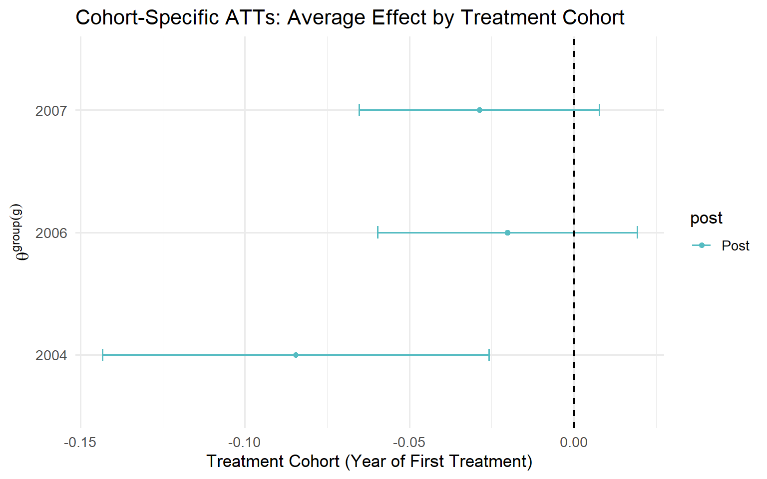
The descending pattern $\hat\theta^{group}(g{=}2) > \hat\theta^{group}(g{=}3) > \hat\theta^{group}(g{=}4)$ is substantively relevant and admits multiple explanations:
- **Accumulated exposure**: Early cohorts have been treated longer, allowing effects to compound.
- **Selection**: Units that adopt earlier may be systematically different (higher motivation, better resources, more favourable context).
- **Macro-institutional context**: The economic or regulatory environment may have shifted between adoption waves, affecting treatment efficacy.
::: {.callout-tip}
**Authors' Recommendation (Callaway & Sant'Anna, 2021).** The `type = "group"` aggregator is the leading choice as the primary measure of global effect. The Overall ATT of **1.488** represents the average effect of participating in the treatment for a typical treated unit, directly analogous to the ATT in the canonical two-period, two-group design, and the most internally coherent summary statistic in staggered settings.
:::
---
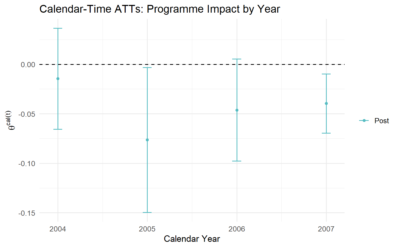
### Aggregation 3: Calendar-Time Effects (`type = "calendar"`)
$$\theta^{cal}(t) = \sum_{g \in \mathcal{G}} \mathbf{1}\{t \geq g\} \cdot P(G = g \mid G \leq t) \cdot ATT(g,\, t)$$
**Business question:** *"What was the aggregate impact of the programme in fiscal quarter $t$?"*
This aggregator maps directly to financial and operational reporting: *"In Q3 2024, the algorithm generated X% margin improvement across all deployed markets."*
```r
agg.ct <- aggte(example_attgt, type = "calendar")
summary(agg.ct)
```
```
Overall summary of ATT's based on calendar time aggregation:
     ATT    Std. Error  [95% Conf. Int.]
  1.4808    0.0347      1.4128  1.5488  *

Time Effects:
  Time  Estimate  Std. Error  [95% Simult. Conf. Band]
  2     0.9209    0.0632      0.7722   1.0697  *
  3     1.5491    0.0496      1.4324   1.6659  *
  4     1.9724    0.0500      1.8547   2.0901  *
```
| $t$ | Contributing Cohorts | Interpretation |
|:----|:---------------------|:---------------|
| $t=2$ | Only $g=2$ (1st year) | Initial effect, only the earliest cohort contributes |
| $t=3$ | $g=2$ (2nd year) + $g=3$ (1st year) | Combines cohort 2 maturation with cohort 3 entry |
| $t=4$ | $g=2$, $g=3$, and $g=4$ | All cohorts contribute, maximum aggregate effect |
: Interpreting the Calendar-Time Effects {.striped}
This aggregator is particularly useful for evaluating the policy's impact in specific fiscal years or for understanding how the aggregate effect evolves as more units receive treatment.
---
### Aggregation 4: Simple ATT (`type = "simple"`)
$$\theta^{simple} = \frac{1}{\kappa} \sum_{g \in \mathcal{G}} \sum_{t \geq g} ATT(g,t) \cdot P(G = g \mid G \leq T)$$
where $\kappa = \sum_{g \in \mathcal{G}} \sum_{t \geq g} P(G = g \mid G \leq T)$ normalises the weights. Each $ATT(g,t)$ cell receives a weight proportional to the cohort's share among ever-treated units times the number of post-treatment periods that cohort contributes, which is why earlier-treated cohorts accumulate more weight.
```
ATT     Std. Error  [95% Conf. Int.]
1.6583  0.0333      1.5931  1.7236  *
```
::: {.callout-warning}
**Limitation of the `simple` aggregator.** `type = "simple"` systematically over-weights early-treated cohorts, because they contribute more post-treatment $(g, t)$ cells and therefore accumulate more weight. This is related to the pathological weighting of TWFE in staggered designs (though the mechanism differs: TWFE uses variance weights while the simple aggregator uses cell-count weights). Use this aggregator only for benchmarking against TWFE or for exploratory sensitivity analysis. It should never be the primary summary of the global treatment effect.
:::
---
### The Aggregation Decision Matrix
| Business Question | Aggregation | `aggte(type=...)` | Role |
|:-----------------|:------------|:------------------|:-----|
| "What was the average effect for a typical treated unit?" | Cohort-specific | `"group"` | Primary |
| "When did effects kick in and how did they evolve?" | Event Study | `"dynamic"` | Complementary |
| "What was the total impact in fiscal year $t$?" | Calendar-time | `"calendar"` | Complementary |
| "How does this compare to a naive TWFE estimate?" | Simple | `"simple"` | Sensitivity only |
---
## Part V: Full R Implementation with Minimum Wage Data {#part-v}
The `did` package ships with county-level employment data from Callaway and Sant'Anna (2021). Several US states increased their minimum wages at different points in time, creating a classic staggered adoption design. This section walks through a complete end-to-end implementation: data preparation, estimation of the $ATT(g,t)$ matrix, pre-trend testing, all four aggregations, and a head-to-head comparison with TWFE.
### Data Preparation
```{r load-data}
# install.packages(c("did", "fixest", "ggplot2", "dplyr", "tidyr",
#                    "scales", "patchwork"))

library(did)
library(fixest)
library(ggplot2)
library(dplyr)
library(tidyr)
library(scales)
library(patchwork)

data(mpdta)
glimpse(mpdta)
```
The `mpdta` dataset contains the following variables:
| Variable | Description |
|:---------|:------------|
| `lemp` | Log county-level teen employment (outcome) |
| `year` | Calendar year (2003–2007) |
| `countyreal` | County identifier |
| `first.treat` | Year of first minimum wage increase (`0` = never treated) |
| `treat` | `1` if county is treated in this year |
: Variables in `mpdta` {.striped}
```{r data-summary}
cat("Number of counties:", n_distinct(mpdta$countyreal), "\n")
cat("Years:", paste(sort(unique(mpdta$year)), collapse = ", "), "\n")
cat("Treatment cohorts:\n")
table(mpdta$first.treat) |> print()
```
```{r explore-data}
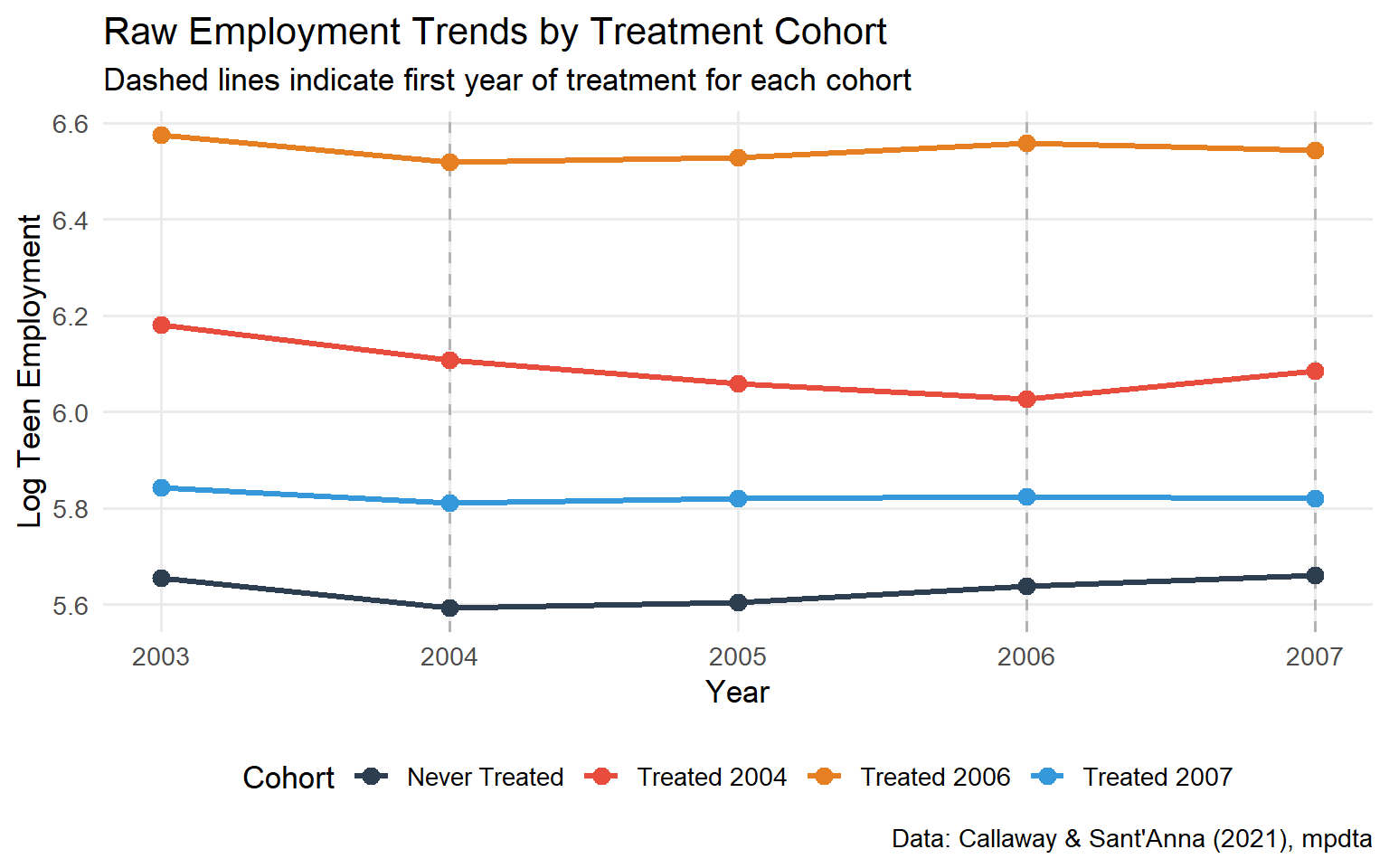
#| fig-cap: "Employment trends by treatment cohort. Pre-treatment trends are broadly similar across groups, providing visual support for parallel trends."
trend_df <- mpdta |>
  mutate(cohort = case_when(
    first.treat == 0    ~ "Never Treated",
    first.treat == 2004 ~ "Treated 2004",
    first.treat == 2006 ~ "Treated 2006",
    first.treat == 2007 ~ "Treated 2007"
  )) |>
  group_by(cohort, year) |>
  summarise(lemp = mean(lemp), .groups = "drop")

ggplot(trend_df, aes(x = year, y = lemp, colour = cohort, group = cohort)) +
  geom_vline(xintercept = c(2004, 2006, 2007),
             linetype = "dashed", colour = "grey70") +
  geom_line(linewidth = 1.2) +
  geom_point(size = 3) +
  scale_colour_manual(values = c(
    "Never Treated" = "#2C3E50",
    "Treated 2004"  = "#E74C3C",
    "Treated 2006"  = "#E67E22",
    "Treated 2007"  = "#3498DB"
  )) +
  labs(
    title    = "Raw Employment Trends by Treatment Cohort",
    subtitle = "Dashed lines indicate first year of treatment for each cohort",
    x = "Year", y = "Log Teen Employment",
    colour = "Cohort",
    caption = "Data: Callaway & Sant'Anna (2021), mpdta"
  ) +
  theme_minimal(base_size = 13) +
  theme(legend.position = "bottom",
        panel.grid.minor = element_blank())
```
### Step 1: Estimate Cohort-Time ATTs with `att_gt()`
```{r att-gt-estimation}
# Verify that lpop covariate is present in the dataset
if (!"lpop" %in% names(mpdta)) stop("Variable 'lpop' not found in mpdta. Check did package version.")

cs_results <- att_gt(
  yname         = "lemp",
  gname         = "first.treat",
  idname        = "countyreal",
  tname         = "year",
  xformla       = ~ lpop,
  data          = mpdta,
  est_method    = "dr",           # Doubly Robust (recommended)
  control_group = "nevertreated",
  bstrap        = TRUE,
  biters        = 1000,
  print_details = FALSE
)

summary(cs_results)
```
```{r plot-att-gt}
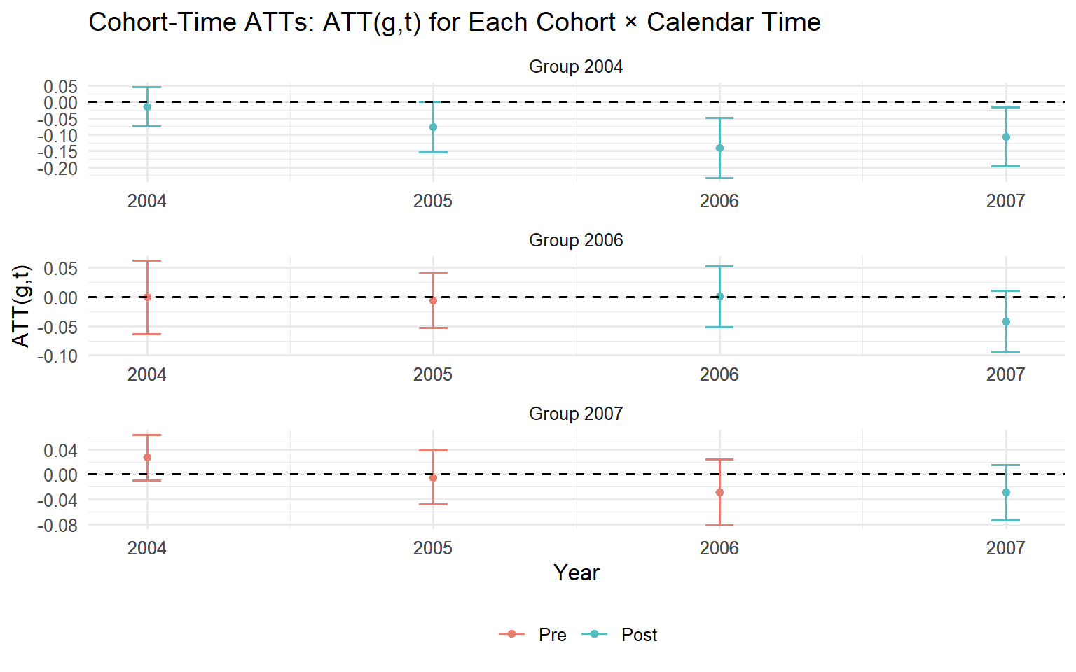
#| fig-cap: "Cohort-time ATT matrix. Pre-treatment cells (event time < 0) test parallel trends, estimates should cluster near zero. Post-treatment cells reveal the causal effects for each cohort at each calendar time."
ggdid(cs_results,
      title  = "Cohort-Time ATTs: ATT(g,t) for Each Cohort × Calendar Time",
      xlab   = "Year",
      ylab   = "ATT(g,t)",
      legend = TRUE) +
  theme_minimal(base_size = 12) +
  theme(legend.position = "bottom")
```
::: {.callout-tip}
**Reading the ATT(g,t) plot.** Each panel corresponds to a treatment cohort $g$. Within each panel, observations to the left of the treatment date (pre-treatment) should be near zero; systematic deviation is evidence against parallel trends. Observations to the right are the causal effect estimates at each post-treatment period.
:::
### Step 2: Pre-Testing Parallel Trends
```{r pretest}
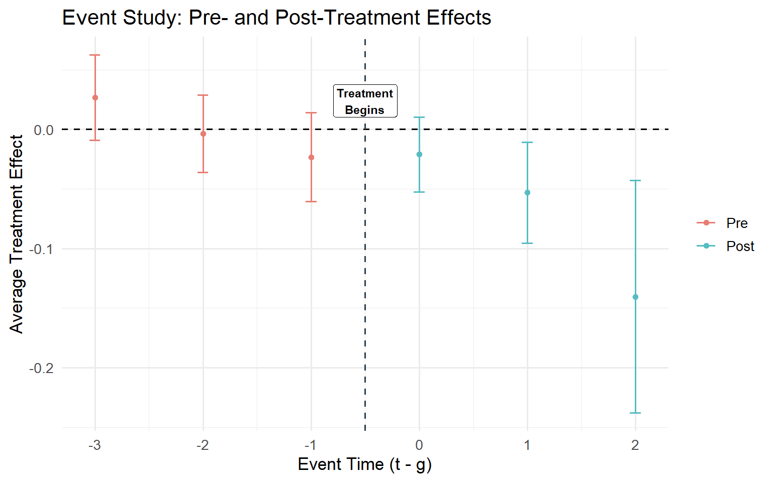
#| fig-cap: "Event study plot including pre-treatment periods. Pre-treatment coefficients should be statistically indistinguishable from zero if parallel trends holds."
es_results <- aggte(cs_results,
                    type  = "dynamic",
                    min_e = -3,
                    max_e = 2,
                    na.rm = TRUE)

summary(es_results)
ggdid(es_results,
      title  = "Event Study: Pre- and Post-Treatment Effects",
      xlab   = "Event Time (t - g)",
      ylab   = "Average Treatment Effect",
      legend = FALSE) +
  geom_vline(xintercept = -0.5, linetype = "dashed", colour = "#2C3E50") +
  annotate("label", x = -0.5,
           y = max(es_results$att.egt, na.rm = TRUE) * 0.9,
           label = "Treatment\nBegins", size = 3, fontface = "bold") +
  theme_minimal(base_size = 13)
```
**Interpreting the pre-test.** Pre-treatment coefficients (event time $< 0$) should be near zero and not statistically significant. Systematic deviations indicate parallel trends violations. The simultaneous confidence bands adjust for multiple testing across all event times; this correction is critical for honest statistical inference, as pointwise bands would understate the uncertainty.
::: {.callout-warning}
**Roth (2022) caution.** A pre-test that passes does not *prove* parallel trends; it merely fails to *reject* it. The pre-test has limited statistical power, particularly in small samples. Moreover, using the pre-test as a decision rule, proceeding only when it passes, stopping when it fails, introduces post-selection bias: the estimates you publish are conditional on having passed the test, which distorts their sampling distribution (Roth 2022). Treat a passing pre-test as one piece of evidence alongside substantive institutional knowledge about why the comparison group provides a valid counterfactual, not as a guarantee.
:::
### Step 3: Event-Study Aggregation
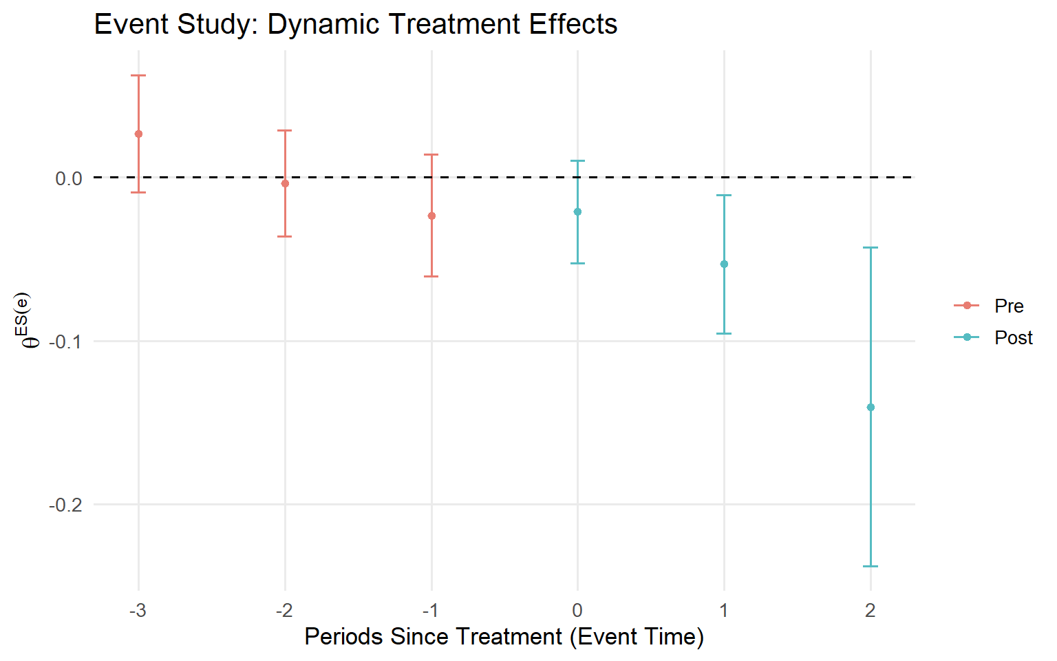
The pre-test above already produced the dynamic aggregation. This step extends it with a dedicated visualisation focused on causal dynamics, using the same estimates (`es_results`) already computed in Step 2 but now emphasising the post-treatment trajectory rather than the pre-trend diagnostic.
```{r event-study}
#| fig-cap: "Event-study aggregation: average effect at each exposure length, aggregated across cohorts. Confidence bands are simultaneous, correcting for multiple testing across event times."
ggdid(es_results,
      title  = "Event Study: Dynamic Treatment Effects",
      xlab   = "Periods Since Treatment (Event Time)",
      ylab   = expression(theta^{ES}(e)),
      legend = FALSE) +
  theme_minimal(base_size = 13) +
  theme(panel.grid.minor = element_blank())
```
### Step 4: Simple Overall ATT
```{r simple-att}
overall_att <- aggte(cs_results,
                     type  = "simple",
                     na.rm = TRUE)
summary(overall_att)
cat(sprintf("\nOverall ATT estimate: %.4f\n", overall_att$overall.att))
cat(sprintf("95%% CI: [%.4f, %.4f]\n",
            overall_att$overall.att - 1.96 * overall_att$overall.se,
            overall_att$overall.att + 1.96 * overall_att$overall.se))
```
### Step 5: Cohort-Specific Effects
```{r cohort-effects}
#| fig-cap: "Cohort-specific ATTs reveal whether earlier or later treatment cohorts experienced different average effects. The descending pattern across cohorts warrants investigation of accumulated exposure, selection, or changing macro context."
group_att <- aggte(cs_results,
                   type  = "group",
                   na.rm = TRUE)

summary(group_att)
ggdid(group_att,
      title  = "Cohort-Specific ATTs: Average Effect by Treatment Cohort",
      xlab   = "Treatment Cohort (Year of First Treatment)",
      ylab   = expression(theta^{group}(g)),
      legend = FALSE) +
  theme_minimal(base_size = 13)
```
### Step 6: Calendar-Time Effects
```{r calendar-effects}
#| fig-cap: "Calendar-time ATTs map the programme's aggregate impact to specific fiscal periods, directly useful for financial reporting and board-level summaries."
calendar_att <- aggte(cs_results,
                      type  = "calendar",
                      na.rm = TRUE)

summary(calendar_att)
ggdid(calendar_att,
      title  = "Calendar-Time ATTs: Programme Impact by Year",
      xlab   = "Calendar Year",
      ylab   = expression(theta^{cal}(t)),
      legend = FALSE) +
  theme_minimal(base_size = 13)
```
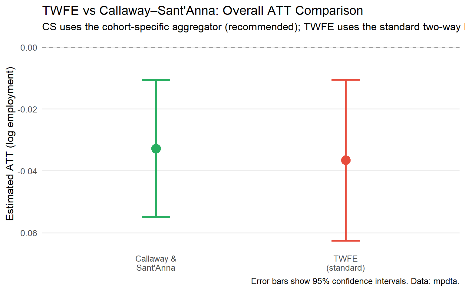
### Step 7: TWFE vs CS: A Direct Comparison
A natural question is: how different is the CS estimate from the TWFE coefficient analysts have been reporting for decades? The code below runs both estimators on the same data and plots the results side by side.
```{r twfe-comparison}
#| fig-cap: "TWFE produces a single coefficient that conflates effects across cohorts, calendar times, and exposure lengths. In this dataset both estimates are negative (minimum wages reduce teen employment), but the magnitude and precision differ, and the TWFE estimate carries no clean heterogeneity breakdown."
mpdta_twfe <- mpdta |>
  mutate(treated_post = as.integer(year >= first.treat & first.treat > 0))

# Note: treated_post collapses all post-treatment periods into a single indicator,
# which does not distinguish dynamic treatment effects. This is a simplified
# TWFE specification designed for benchmarking purposes and is not directly
# comparable to the cohort-time ATT(g,t) estimates from CS.
twfe_fit <- feols(lemp ~ treated_post | countyreal + year,
                  data    = mpdta_twfe,
                  cluster = ~countyreal)

twfe_coef <- coef(twfe_fit)["treated_post"]
twfe_se   <- se(twfe_fit)["treated_post"]
cs_coef   <- group_att$overall.att
cs_se     <- group_att$overall.se

comparison_df <- tibble(
  Method   = c("TWFE\n(standard)", "Callaway &\nSant'Anna"),
  Estimate = c(twfe_coef, cs_coef),
  SE       = c(twfe_se, cs_se),
  Lower    = c(twfe_coef - 1.96 * twfe_se, cs_coef - 1.96 * cs_se),
  Upper    = c(twfe_coef + 1.96 * twfe_se, cs_coef + 1.96 * cs_se)
)

ggplot(comparison_df, aes(x = Method, y = Estimate, colour = Method)) +
  geom_hline(yintercept = 0, linetype = "dashed", colour = "grey50") +
  geom_point(size = 5) +
  geom_errorbar(aes(ymin = Lower, ymax = Upper), width = 0.15, linewidth = 1.2) +
  scale_colour_manual(values = c(
    "TWFE\n(standard)"      = "#E74C3C",
    "Callaway &\nSant'Anna" = "#27AE60"
  )) +
  labs(
    title    = "TWFE vs Callaway–Sant'Anna: Overall ATT Comparison",
    subtitle = "CS uses the cohort-specific aggregator (recommended); TWFE uses the standard two-way FE regression",
    y        = "Estimated ATT (log employment)",
    x        = NULL,
    caption  = "Error bars show 95% confidence intervals. Data: mpdta."
  ) +
  theme_minimal(base_size = 13) +
  theme(legend.position     = "none",
        panel.grid.minor    = element_blank(),
        panel.grid.major.x  = element_blank())
```
---
## Part VI: A Diagnostic Checklist for Practitioners {#part-vi}
Before presenting any DiD analysis to leadership, verify the following across three dimensions: research design, estimation, and reporting.
### Design Checklist
- [ ] **Control cohort defined and justified**: Is the comparison group plausibly on the same outcome trend as the treated cohort in the absence of treatment?
- [ ] **Parallel trends assessed**: Both via institutional knowledge *and* empirical pre-trends test.
- [ ] **No anticipation evaluated**: Did units change behaviour before treatment formally began?
- [ ] **SUTVA considered**: Could treated units contaminate the control group via spillovers or general equilibrium effects?
### Estimation Checklist
- [ ] **CS estimator used** (not TWFE) when staggered adoption and heterogeneous effects are plausible. TWFE remains acceptable when treatment effects are homogeneous or all units are treated simultaneously.
- [ ] **Covariates included** if cohorts differ in pre-treatment characteristics that drive outcome trends.
- [ ] **Doubly robust estimator selected** (`est_method = "dr"`) unless there is a specific reason to prefer OR or IPW alone.
- [ ] **Comparison group choice documented**: `nevertreated` vs `notyettreated`, and the rationale for the choice.
- [ ] **Multiplier bootstrap used** for simultaneous confidence bands across event times.
### Reporting Checklist
- [ ] **ATT(g,t) heatmap** presented, or at minimum by-cohort event studies.
- [ ] **Pre-trends diagnostic** explicitly reported with coefficient estimates and joint test p-values.
- [ ] **Aggregation method stated and justified**: which business question is being answered?
- [ ] **TWFE comparison provided** as a robustness and benchmarking check.
- [ ] **Sensitivity analysis discussed**: how robust are conclusions to modest violations of parallel trends?
### When to Stop
Some conditions should trigger reassessment before proceeding:
| Red Flag | Implication |
|:---------|:-----------|
| Pre-treatment ATTs are large and statistically significant | Parallel trends likely violated; results not credible |
| Nearly all units eventually treated and comparison group is tiny | Low power; consider Synthetic Control instead |
| Massive spillovers from treated to control units | ATT underestimated; redesign the comparison group |
| Treatment turns on and off across periods | Standard CS framework not applicable; consider de Chaisemartin & D'Haultfoeuille (2020) |
: Conditions that should trigger reassessment before proceeding {.striped}
---
## Part VII: Five Questions for Your Analytics Team {#part-vii}
If your organisation is using DiD to evaluate strategic initiatives, these five questions will quickly reveal whether the analysis is methodologically sound.
**1. "Did you use TWFE or a modern staggered DiD estimator?"**
If the team ran a TWFE regression on a staggered rollout, the estimate may be biased when treatment effects vary across cohorts or over time. Ask for the Goodman-Bacon decomposition to see how much weight comes from contaminated comparisons (late-treated units against already-treated units).
**2. "Can you show me the ATT(g,t) matrix?"**
If they can only show a single coefficient, all heterogeneity information is hidden. Modern DiD should show effects by cohort and by exposure duration. A single number is a starting point, not a conclusion.
**3. "What does the pre-trend test show?"**
Not just "it looks parallel": what are the actual coefficient estimates for pre-treatment periods? What is the p-value for the joint test that all pre-treatment coefficients are zero? Are simultaneous bands (not pointwise) being used?
**4. "What does the event study tell us about dynamics?"**
A positive effect at $e=0$ that grows to a larger effect at $e=4$ is a very different strategic story than a large effect at $e=0$ that decays to zero by $e=4$. The first suggests a programme that takes time to mature; the second, one that is effective only for early adopters or fades with habituation. TWFE cannot distinguish these narratives. The CS event study can.
**5. "How sensitive are the conclusions to violations of parallel trends?"**
Under the HonestDiD framework (Rambachan & Roth, 2023), you can bound conclusions under specified violations. If the "the programme worked" finding holds even when parallel trends is violated by 50% of its magnitude, you have a robust result. If it collapses under a 5% violation, caution is warranted regardless of the pre-test outcome.
---
## Conclusion: From Statistical Methodology to Competitive Advantage
The organisations that will win in the next decade are not those with the most data. They are those with the best **causal models**: the ability to know with confidence what actually drives results, and therefore where to invest next.
Modern DiD, particularly the Callaway and Sant'Anna estimator, is not a technical refinement for academic purists. It is a practical tool that:
- Produces estimates with unambiguous economic interpretations: $ATT(g,t)$ means what it says
- Uses more transparent, researcher-controlled weighting schemes (cohort size, not statistical variance), though some aggregators such as calendar-time still involve implicit weights that should be interpreted carefully
- Provides honest pre-testing that does not rely on contaminated comparisons
- Delivers doubly robust inference that protects against common modelling errors
- Enables heterogeneity analysis that can reshape targeting and rollout strategy
That said, TWFE remains valid when treatment effects are homogeneous across cohorts and time, or when all units are treated simultaneously. The CS framework is not a blanket replacement; it is the right tool when the standard assumptions behind TWFE are implausible, which in staggered settings they usually are.
Two closely related alternatives are worth noting for practitioners: Sun & Abraham (2021) propose an interaction-weighted estimator that is asymptotically equivalent to CS but estimated within a single regression framework, which some practitioners find more familiar; and de Chaisemartin & D'Haultfœuille (2020) extend the analysis to settings where treatment can be turned on and off across periods.
The `did` package makes this accessible to any analyst who can run a regression. The question is not whether you can afford to use modern methods. It is whether you can afford not to.
---
## References {#references .unnumbered}
Baker, A., Callaway, B., Cunningham, S., Goodman-Bacon, A., & Sant'Anna, P. H. C. (2026). Difference-in-differences designs: A practitioner's guide. *Journal of Economic Literature*, 64(2), 498–557.
Callaway, B., & Sant'Anna, P. H. C. (2021). Difference-in-Differences with multiple time periods. *Journal of Econometrics*, 225(2), 200–230. <https://doi.org/10.1016/j.jeconom.2020.12.001>
de Chaisemartin, C., & D'Haultfœuille, X. (2020). Two-way fixed effects estimators with heterogeneous treatment effects. *American Economic Review*, 110(9), 2964–2996.
Goodman-Bacon, A. (2021). Difference-in-Differences with variation in treatment timing. *Journal of Econometrics*, 225(2), 254–277.
Holland, P. W. (1986). Statistics and causal inference. *Journal of the American Statistical Association*, 81(396), 945–960.
Rambachan, A., & Roth, J. (2023). A more credible approach to parallel trends. *Review of Economic Studies*, 90(5), 2555–2591.
Roth, J. (2022). Pre-test with caution: Event-study estimates after testing for parallel trends. *American Economic Review: Insights*, 4(3), 305–322.
Roth, J., Sant'Anna, P. H. C., Bilinski, A., & Poe, J. (2023). What's trending in difference-in-differences? A synthesis of the recent econometrics literature. *Journal of Econometrics*, 235(2), 2218–2244.
Sant'Anna, P. H. C., & Zhao, J. (2020). Doubly robust difference-in-differences estimators. *Journal of Econometrics*, 219(1), 101–122.
Sun, L., & Abraham, S. (2021). Estimating dynamic treatment effects in event studies with heterogeneous treatment effects. *Journal of Econometrics*, 225(2), 175–199.