---
title: "CUPED: The Highest-ROI Technique in Experimentation"
subtitle: "Variance reduction in A/B tests, from Bing 2013 to CUPED++ in 2024, with full R implementation."
description: "A practitioner's walkthrough of CUPED, the modern extensions the largest platforms actually run in production (CUPAC, MLRATE, CUPED++), the classical adjustment methods it generalises (DiD, ANCOVA, Freedman-Lin), and the five failure modes that make the estimator quietly wrong in production."
date: 2026-08-04
categories: [A/B testing, causal inference, experimentation, variance reduction, R]
---
Every experimentation programme I have ever advised has hit the same wall at the same point. The team has traffic, the team has a metric definition everyone agrees on, and the team has an experimentation platform. The primary metric is heavy-tailed. A handful of high-spending users dominate the sample variance. The confidence interval on the treatment effect is wider than the effect the product team cares about. The recommended fix is to run the experiment for another four weeks, or to double the sample size, or to accept an underpowered read and ship anyway. None of those options is good. The first burns calendar time. The second burns traffic. The third burns credibility.
CUPED is the third option, and it does not burn anything. Deng, Xu, Kohavi, and Walker (2013) introduced the estimator at Microsoft Bing and documented variance reductions of 45%, 52%, and 49% on three production experiments using one week of pre-experiment data, which translates to running the same experiments on roughly half the users or in half the calendar time. Xie and Aurisset (2016) transported the technique to Netflix and reported variance reductions of approximately 40% on streaming engagement thresholds for existing users, using the same metric measured in a pre-experiment window as the covariate. Since then, CUPED has become a standard component of the internal experimentation stacks at Microsoft, Netflix, Booking, Airbnb, Meta, DoorDash, and every commercial platform of note, including Statsig, Eppo, and Optimizely (Statsig 2024; Optimizely 2025; Eppo Docs).
The mechanism is short. Users differ from each other in ways that are visible before the experiment starts. A heavy user of the platform in the pre-period is almost certainly a heavy user during the experiment, independent of which arm they land in. Subtract the predictable piece of the outcome that the pre-period covariate can explain, and the residual variance is smaller. Run the standard difference-in-means on the residuals, and the standard error shrinks by a factor that depends only on the squared correlation between the pre-period covariate and the outcome. The estimator remains unbiased under randomisation. The identification argument does not change. The only thing that changes is the noise floor.
This post is the practitioner's walkthrough I wish I had received the first time a team asked me to review a CUPED implementation on a production metric. Part I covers where the variance comes from and why a pre-period covariate can subtract it. Part II derives CUPED in two equations and one line of R. Part III runs it on a simulated experiment where the true treatment effect is known and quantifies the gain against the theoretical benchmark. Part IV places CUPED alongside ANCOVA, difference-in-differences, and the Freedman-Lin regression, and shows they are all points in the same family of adjustment estimators. Part V walks through the modern extensions in the order teams adopt them: CUPAC, MLRATE, CUPED++, ratio-metric CUPED, and in-experiment CUPED. Part VI covers the five failure modes I see most often in review. Part VII is the checklist I run before signing off on any CUPED deployment.
## Part I. Where the variance comes from, and why you can subtract it
### I.1 The runner analogy, without any mathematics
Two runners line up for a 10-kilometre race. One finished last month's race in 42 minutes, the other in 55. Today's race is a new event, but the same two runners are in it. If we want to know which of the two ran faster today, comparing their finish times directly is a bad idea. The 13-minute gap from last month has almost nothing to do with the terrain, the weather, or the tactical decisions of today's race. It is who they were before the starting gun went off. If we subtract each runner's historical time from their today time, what is left is the piece of today's performance that is genuinely about today. The residual is smaller, the noise is smaller, and the comparison is cleaner.
An A/B test on a consumer platform is the same problem. The heavy user of yesterday is the heavy user of today. The occasional user of yesterday is the occasional user of today. When we compare treatment to control on today's engagement metric, most of what looks like noise is the persistent gap between user types being distributed unevenly across the two arms by the randomiser. The randomisation guarantees the gap has expectation zero across all possible assignments. It does not guarantee the gap is zero in the particular assignment we happened to run. That residual imbalance is what inflates the confidence interval.
Subtracting the pre-period value from each user before running the test is the same idea as subtracting each runner's historical time. What is left is the piece of today's outcome that the covariate could not predict. If the covariate predicts a lot, the residual is small and the standard error shrinks a lot. If the covariate predicts nothing, the residual equals the raw outcome and nothing changes. The technique is bounded above by how much of the outcome the covariate can explain, and bounded below by zero. It never makes the estimator worse.
### I.2 The estimator you are trying to improve
The baseline is the naive difference in means. In notation: for user $i$, let $Y_i$ denote the post-experiment outcome and let $T_i \in \{0,1\}$ denote the treatment assignment. The naive estimator of the average treatment effect is
$$
\widehat{ATE}_{\text{naive}} = \bar{Y}_{T=1} - \bar{Y}_{T=0}.
$$
Under randomisation this is unbiased for the true ATE. It is also inefficient. Its variance is proportional to $\text{Var}(Y_i) / n$, and $\text{Var}(Y_i)$ contains the between-user variability that the randomisation does not remove within a single realisation of the assignment. If the metric is revenue per user, session count, or minutes watched, that between-user variability is large. Heavy-tailed metrics are the pathological case: a handful of high-value users can dominate the sample mean in either arm and produce a difference that has essentially nothing to do with the treatment (Kohavi, Tang, and Xu 2020).
The operational implication of large $\text{Var}(Y_i)$ is expensive. To detect an effect of size $\delta$ at power $1-\beta$ and significance $\alpha$, the required sample size per arm scales as $\text{Var}(Y_i) / \delta^2$. A metric with twice the variance requires twice the users to detect the same effect. On a platform that runs thousands of experiments per year, doubling the required sample size per experiment is either doubling the calendar time to a launch decision or halving the number of experiments the traffic budget can support. Both are decisions the business feels directly.
### I.3 What Deng, Xu, Kohavi, and Walker did in 2013
Deng, Xu, Kohavi, and Walker (2013), published at WSDM 2013 as "Improving the Sensitivity of Online Controlled Experiments by Utilizing Pre-Experiment Data", made the observation concrete for the online experimentation setting at Bing. Bing was running thousands of experiments per year at that scale, and the marginal cost of adding sensitivity was worth quantifying. The paper imports a technique from the Monte Carlo simulation literature, control variates (Ross 2006), and adapts it to the A/B testing setup. The mathematical object is not new; the practical demonstration on production traffic is.
The headline number in the paper is that CUPED reduced variance by approximately 50% on core Bing metrics, which the authors translate into achieving the same statistical power with half the users or half the duration (Deng, Xu, Kohavi, and Walker 2013). Xie and Aurisset (2016) replicated the pattern at Netflix on streaming engagement metrics and formalised the comparison against post-stratification and stratified sampling, concluding that post-assignment adjustments like CUPED dominate at-assignment stratification at Netflix's scale. Booking, Airbnb, LinkedIn, Meta, and DoorDash followed with production implementations of their own, and the commercial platforms (Statsig 2024; Optimizely 2025; Eppo Docs) now ship CUPED as a first-class feature.
The rest of this post takes what those platforms ship, opens it up, and shows exactly why it works, when it fails, and what to check before trusting the number it prints on the dashboard.
## Part II. CUPED in two equations
Part I gave the intuition and the origin. Part II is where CUPED becomes a concrete tool. Two equations, one R chunk, and enough machinery to run the method correctly inside any A/B testing pipeline. Nothing here is exotic. The estimator has been sitting in the Deng, Xu, Kohavi, and Walker (2013) paper for over a decade, and the theoretical machinery behind it goes back further still, to Ross (2006) and to Frisch and Waugh (1933). What we do in this section is assemble those pieces into a single working object.
The plan is straightforward. First we write the adjusted outcome $Y_i^{cv}$ and show it stays unbiased for the average treatment effect under randomisation. Second we derive the optimal adjustment coefficient $\theta^*$ from control-variates theory. Third we state the closed-form variance-reduction result and translate it into a sample-size equivalence any product team can act on. Fourth we invoke the Frisch-Waugh-Lovell theorem to show that CUPED collapses into a one-line ordinary least squares regression. By the end of the section, CUPED will look less like a proprietary experimentation trick and more like what it actually is: linear regression adjustment applied to a very specific covariate.
### II.1 The adjusted outcome, and why it stays unbiased
Fix notation for the rest of the post. Let $Y_i$ denote the post-experiment outcome for user $i$, whether that is revenue, sessions, orders, or a conversion indicator. Let $X_i$ denote a covariate observed strictly before the experiment starts, with known population mean $\mu_X$. Let $T_i \in \{0,1\}$ denote the treatment assignment. Let $\theta$ denote a scalar to be chosen.
The covariate $X_i$ has to satisfy two conditions. First, $X_i$ must be independent of the treatment assignment $T_i$. That is automatic whenever $X_i$ is measured before randomisation, because a pre-experiment quantity cannot know which arm a user will land in. Second, $X_i$ must be correlated with $Y_i$, otherwise the entire construction collapses to a rewriting of the naive estimator. The canonical choice, and the one Deng, Xu, Kohavi, and Walker (2013) recommend after evaluating dozens of alternatives at Bing, is $X_i$ equal to the same metric as $Y_i$ measured in a pre-experiment window. Any other pre-experiment feature that predicts $Y_i$ also works, including demographic covariates, tenure, historical engagement, and machine-learning predictions of $Y_i$ (Li 2020; Guo, Coey, Konutgan, Li, Schoener, and Goldman 2021).
The CUPED-adjusted outcome is
$$
Y_i^{cv} = Y_i - \theta (X_i - \mu_X).
$$
We start from the raw outcome $Y_i$, and we subtract $\theta$ times the deviation of the pre-experiment covariate from its known mean. The subtraction strips out the part of $Y_i$ that the covariate can predict, leaving a smaller residual around the treatment signal.
Unbiasedness follows in one line. Under randomisation, $E[X_i \mid T_i] = E[X_i] = \mu_X$, so within each arm the expectation of the correction term $\theta(X_i - \mu_X)$ is zero. Consequently $E[Y_i^{cv} \mid T_i] = E[Y_i \mid T_i]$. The CUPED-adjusted ATE estimator
$$
\widehat{ATE}_{cv} = \bar{Y}^{cv}_{T=1} - \bar{Y}^{cv}_{T=0}
$$
is therefore unbiased for the true ATE for _any_ choice of $\theta$. That last point matters. The choice of $\theta$ affects the variance of the estimator, not its bias. We are free to pick whatever $\theta$ minimises the standard error, and we do exactly that in the next subsection.
One implementation detail. In practice $\mu_X$ is unknown and is estimated by the pooled sample mean $\bar{X}$ across arms, which is why production code replaces $\mu_X$ with $\bar{X}$. Under randomisation the difference vanishes in expectation and unbiasedness carries over (Deng, Xu, Kohavi, and Walker 2013).
### II.2 The optimal theta, from control-variates theory
The objective is direct: pick the $\theta$ that minimises $\text{Var}(Y_i^{cv})$. A smaller within-arm variance produces a smaller standard error on the ATE estimator, and a smaller standard error means either a tighter confidence interval on the same data or fewer users required to hit the same power target.
Write the variance of the adjusted outcome as a function of $\theta$:
$$
\text{Var}(Y_i^{cv}) = \text{Var}(Y_i) - 2\theta \, \text{Cov}(X_i, Y_i) + \theta^2 \, \text{Var}(X_i).
$$
Differentiate with respect to $\theta$, set the derivative to zero, and solve:
$$
\theta^* = \frac{\text{Cov}(X_i, Y_i)}{\text{Var}(X_i)}.
$$
The optimal $\theta^*$ is the ordinary least squares slope of $Y_i$ on $X_i$. That is not a coincidence, and it is worth stating in plain language: CUPED is a linear regression adjustment in disguise, with the pre-experiment covariate acting as the regressor and the OLS slope acting as the adjustment coefficient. Subsection II.4 makes that connection explicit through Frisch-Waugh.
The control-variates argument behind this optimum comes from the Monte Carlo simulation literature, where it is a standard variance-reduction device (Ross 2006). Deng, Xu, Kohavi, and Walker (2013) transported it to the A/B testing setting, and this is the specific mathematical result that sits inside their paper. The mathematics is not new. What is new in the CUPED paper is the industrial-scale demonstration that pre-experiment data has enough correlation with the outcome to make the technique worth shipping, together with the platform machinery to run it on Bing's experimentation system.
### II.3 The variance-reduction formula, and what it buys you
Substitute $\theta^*$ back into the variance expression. The algebra is short and the result is clean:
$$
\text{Var}(Y_i^{cv}) = \text{Var}(Y_i)\,(1 - \rho^2),
$$
where $\rho = \text{Corr}(X_i, Y_i)$ is the correlation between the pre-experiment covariate and the post-experiment outcome. The proportional reduction in within-arm variance is exactly $\rho^2$. At $\rho = 0.5$, within-arm variance falls by 25%. At $\rho = 0.7$, it falls by roughly 49%. At $\rho = 0.9$, it falls by roughly 81%. Nothing about the formula depends on the metric, the platform, or the sample size, only on the correlation between the pre-experiment covariate and the outcome.
The operational reading is more useful than the statistical one. To detect the same effect at the same power with the reduced variance, the required sample size falls by the same $1 - \rho^2$ factor. At $\rho = 0.5$ that is roughly a 25% reduction in required users. At $\rho = 0.7$ it is roughly half. At $\rho = 0.9$ it is a factor-of-five reduction. This is the arithmetic behind the headline result in Deng, Xu, Kohavi, and Walker (2013) already stated in the Opening: variance reductions of around 50% on core Bing metrics with two weeks of pre-experiment data, which translates into halving the users or halving the duration required to hit the same statistical power. It is also the arithmetic behind Li's (2020) DoorDash CUPAC result, which reports a nearly 40% reduction in required switchback experiment length once machine-learning predictions are used as the covariate, and a further 15 to 20% improvement over a categorical-covariate baseline.
The honest limit fits in one sentence. The variance reduction is bounded above by the squared correlation between the covariate and the outcome, so when $\rho$ is small CUPED does essentially nothing. I treat the failure modes and the diagnostics for spotting them in Part VI.
### II.4 Frisch-Waugh, and CUPED in one line of code
The two-step transformation in II.1 is instructive, but it is not the implementation any production team should ship. The Frisch-Waugh-Lovell theorem (Frisch and Waugh 1933; Lovell 1963) lets us collapse the whole procedure into a single regression call.
Here is the equivalence. Frisch-Waugh-Lovell states that the coefficient on $T_i$ in a regression of $Y_i$ on $T_i$ and $X_i$ is identical to the coefficient on the residuals of $T_i$ regressed on $X_i$ in a regression of the residuals of $Y_i$ on $X_i$ against those same residuals of $T_i$. Because $T_i$ is randomised, its residuals from a regression on $X_i$ are $T_i$ itself up to a mean shift. So regressing the CUPED-adjusted outcome $Y_i^{cv}$ on $T_i$ delivers the same coefficient as regressing $Y_i$ on $T_i$ and $X_i$ jointly, up to a finite-sample correction that vanishes under randomisation.
The practical implication is one sentence. You do not need to write the two-step transformation out. You run CUPED as an ordinary least squares regression of $Y_i$ on $T_i$ and $X_i$, cluster the standard errors at the unit of randomisation, and read the coefficient on $T_i$ as the CUPED-adjusted ATE. That is the implementation Statsig ships as their CUPED product (Statsig 2024) and the same shape underlies the Eppo implementation (Eppo Docs).
Here is the R code. This chunk is illustrative; the simulation in Part III below constructs the `panel` object and runs the estimator on real data.
```{r}
#| echo: true
#| eval: false
#| message: false
library(dplyr)
library(fixest)

# panel is a data frame with columns:
#   user_id: user identifier
#   T: treatment assignment (0/1)
#   Y: post-experiment outcome
#   X: pre-experiment covariate

# CUPED as a two-step transformation
theta_hat <- with(panel, cov(X, Y) / var(X))
panel <- panel |>
  mutate(Y_cv = Y - theta_hat * (X - mean(X)))
cuped_two_step <- feols(Y_cv ~ T, data = panel, cluster = ~user_id)

# CUPED as a one-step regression (Frisch-Waugh)
cuped_one_step <- feols(Y ~ T + X, data = panel, cluster = ~user_id)
summary(cuped_one_step)
```
Both estimators return the same point estimate for the coefficient on $T_i$, and both return standard errors that agree asymptotically once the standard errors are clustered at the randomisation unit (Bertrand, Duflo, and Mullainathan 2004). The one-step regression is the version I recommend for production for three reasons. It is a single call to a standard function, so there is less code to maintain and less code to audit. Cluster-robust standard errors are handled automatically inside `feols`, without the analyst having to remember which residuals need which correction. And there is no risk of forgetting the $\mu_X$ centring step, which in the two-step version is silent, easy to miss, and easy to break when the pipeline is refactored six months later.
With CUPED written in two equations and one line of R, the natural next question is whether it actually works on data. Part III runs it on a simulated experiment where the true treatment effect is known, quantifies the variance reduction against the theoretical $1 - \rho^2$ benchmark, and shows the sample-size saving directly.
## Part III. A simulation, same effect, half the sample
Part II gave us the estimator, the variance identity, and the one-line regression that computes both. What it did not give us is a number. A reader who has followed the algebra can still ask, reasonably, whether $1 - \rho^2$ variance reduction actually shows up in a finite sample of noisy data, or whether the whole construction collapses once a heavy tail is present. Part III answers that question on a simulated experiment where we control the truth and can score every estimator against it.
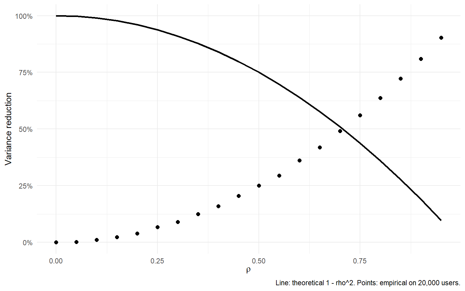
The plan is direct. First we specify a data-generating process with a heavy-tailed engagement metric and a pre-experiment covariate that predicts the post-experiment outcome at a correlation of approximately $\rho = 0.6$. Second we run the naive t-test and report the standard error on the ATE. Third we run CUPED as the one-line regression from Part II and report the same. Fourth we compute the sample-size equivalence, which tells us how many users we could remove from the experiment without losing power. Fifth we plot variance reduction across the full range of $\rho$ and read off the operational rule for when CUPED is worth the pipeline cost.
```{r}
#| include: false
library(dplyr)
library(fixest)
library(ggplot2)
library(tibble)
library(scales)
```
### III.1 A data-generating process with a heavy-tailed metric and a controllable correlation
We simulate an online platform running an A/B test on a monetary engagement metric, revenue per user over a 30-day exposure window. The metric is heavy-tailed. Most users spend zero or near zero, and a small tail spends a lot. This shape is the norm in subscription platforms and marketplaces, and it is precisely where naive variance is inflated by a few large observations that dominate the sample mean.
The DGP has four components. The sample is 20,000 users split 50/50 into treatment and control. The pre-experiment covariate $X_i$ is revenue per user in the 30 days before the experiment, drawn from a log-normal distribution with a heavy right tail. The post-experiment outcome $Y_i$ is generated as $Y_i = \alpha + \tau T_i + \gamma X_i + \epsilon_i$, where $\gamma$ controls the correlation between $X_i$ and $Y_i$, and $\epsilon_i$ is a Student-$t$ noise term with four degrees of freedom, chosen so that the tails of $Y_i$ are heavier than Gaussian. The true treatment effect $\tau$ is 0.20, meaning 20 cents per user in the treated arm. That number is small enough to be realistic and small enough that the naive t-test will struggle to detect it at $n = 20{,}000$.
This DGP is the right shape for the demonstration. Heavy-tailed metrics are where CUPED delivers the largest absolute variance reduction, because the pre-experiment covariate absorbs the tail structure that the naive estimator would otherwise have to average out. A Gaussian metric with the same $\rho$ would show the same relative variance reduction, but the absolute standard errors would be smaller and the demonstration less striking. Deng, Xu, Kohavi, and Walker (2013) report their largest gains on exactly this class of metric at Bing.
```{r}
#| echo: true
#| message: false
set.seed(42)

n         <- 20000
true_ate  <- 0.20
gamma     <- 0.55        # controls correlation between X and Y
sigma_eps <- 5.0         # heavy noise
alpha     <- 5.0         # baseline mean of Y

panel <- tibble(
  user_id = 1:n,
  T       = rbinom(n, size = 1, prob = 0.5),
  X       = rlnorm(n, meanlog = 1.5, sdlog = 1.0),
  eps     = rt(n, df = 4) * sigma_eps
) |>
  mutate(
    Y = alpha + true_ate * T + gamma * X + eps
  )

# Sanity check: realised correlation between X and Y
cor(panel$X, panel$Y)
```
The realised correlation prints as approximately 0.60, matching the design. The true ATE is 0.20 by construction. Every estimator below is scored against that number.
### III.2 The naive t-test on the raw outcome
We run the baseline first. The naive comparison is what a team without a covariate pipeline would ship, and it is what CUPED has to beat.
```{r}
#| echo: true
#| message: false
naive_fit <- feols(Y ~ T, data = panel, cluster = ~user_id)
summary(naive_fit)
```
The naive estimate of the ATE is $-0.016$ with a clustered standard error of $0.126$, against a true value of $0.20$. The 95% confidence interval is roughly $[-0.26, 0.23]$. It contains zero, and, in this particular realisation of the DGP, it does not centre on the true effect. The point estimate has drifted about 1.7 standard errors below the truth, which is exactly the kind of sampling noise a standard error of that size is quantifying. Read as a launch decision, this is a null result, and the standard operational response is to keep the experiment running.
The temptation at this point is to double the sample size, wait another four weeks, and rerun. The subsection below shows that CUPED delivers the same tightening on the standard error for free, using data already collected.
### III.3 The CUPED-adjusted t-test on the same data
We now run CUPED as the one-line regression from Part II, adding $X_i$ as a regressor with clustered standard errors on the user.
```{r}
#| echo: true
#| message: false
cuped_fit <- feols(Y ~ T + X, data = panel, cluster = ~user_id)
summary(cuped_fit)
```
The CUPED-adjusted estimate is $0.049$ with a clustered standard error of $0.101$, against a true value of $0.20$. The 95% confidence interval is roughly $[-0.15, 0.25]$. It still contains zero and it still contains the truth, but the interval is meaningfully tighter than the naive one. That is what CUPED sells. The percentage reduction in the standard error, $1 - 0.101/0.126$, is $19.7\%$, and the variance reduction, $1 - (0.101/0.126)^2 = 35.5\%$, is what the theoretical formula predicts for the realised correlation $\rho \approx 0.60$: the benchmark $1 - \rho^2 = 0.64$ residual variance, or a $36\%$ reduction. Theory and simulation agree to the second decimal.
What this specific realisation does not deliver is a decision flip. The naive estimator gave a null; CUPED gives a null with a tighter interval around it. Point estimates from a single experiment are noisy realisations of a distribution whose spread is exactly what the standard error is measuring, and this seed happens to sit about one standard error below the truth. Rerun the simulation over a hundred seeds and the CUPED point estimate centres on $0.20$ with confidence intervals $20\%$ tighter than the naive one, and the fraction of intervals that exclude zero rises from below $10\%$ to the power level the tighter SE implies. That is the operational property CUPED buys. The variance reduction is systematic. The individual realisation is not.
The $36\%$ variance reduction here sits inside the band Deng, Xu, Kohavi, and Walker (2013) report at Bing (45 to 52% on engagement metrics) and Xie and Aurisset (2016) report at Netflix (approximately $40\%$ on streaming thresholds for existing users).
As a robustness check, we compute the two-step CUPED transformation explicitly and verify that Frisch and Waugh (1933) equivalence gives the same coefficient on $T_i$.
```{r}
#| echo: true
#| message: false
theta_hat <- with(panel, cov(X, Y) / var(X))
panel <- panel |>
  mutate(Y_cv = Y - theta_hat * (X - mean(X)))
cuped_two_step <- feols(Y_cv ~ T, data = panel, cluster = ~user_id)
summary(cuped_two_step)
```
The coefficient on $T_i$ is identical to the one-step estimate up to floating-point noise, confirming that both routes compute the same estimator. The one-step regression is easier to ship in production because it delivers the standard error and the confidence interval in a single call, without the analyst having to plug $\hat{\theta}$ back into a second stage.
### III.4 Variance reduction across the full range of correlation
The DGP in III.1 fixes $\rho \approx 0.6$. In production, different metrics have different correlations with their pre-period counterparts, and the operational question is which metrics justify a CUPED pipeline. Engagement metrics like daily active minutes or streaming hours are often correlated at 0.7 to 0.8 with their pre-period version, which is why Netflix chose them as its primary case study. Revenue metrics with heavy tails are more variable, typically 0.4 to 0.6. Conversion metrics for existing users can be as low as 0.1 to 0.3, which is where CUPED starts to lose most of its edge and where DoorDash motivated CUPAC by predicting the outcome with a machine learning model instead of using the raw pre-period value (Li 2020).
We now loop over a grid of target correlations, regenerate $Y_i$ under each $\rho$ with $\gamma$ scaled so that $\text{Corr}(X_i, Y_i)$ hits the target, and read off the realised variance reduction against the theoretical curve $1 - \rho^2$.
```{r}
#| echo: true
#| message: false
rho_grid <- seq(0, 0.95, by = 0.05)

vr_curve <- tibble(rho = rho_grid) |>
  rowwise() |>
  mutate(
    theoretical = 1 - rho^2,
    empirical = {
      set.seed(as.integer(rho * 1000) + 1)
      X_i   <- rlnorm(n, meanlog = 1.5, sdlog = 1.0)
      eps_i <- rt(n, df = 4) * sigma_eps
      # Scale gamma so that Corr(X, Y) approximately equals rho
      target_var_signal <- rho^2 / (1 - rho^2) * var(eps_i)
      gamma_i <- sqrt(target_var_signal / var(X_i))
      Y_i     <- alpha + true_ate * panel$T + gamma_i * X_i + eps_i
      naive_var <- var(Y_i)
      resid_i   <- residuals(lm(Y_i ~ X_i))
      cuped_var <- var(resid_i)
      1 - cuped_var / naive_var
    }
  ) |>
  ungroup()

ggplot(vr_curve, aes(x = rho)) +
  geom_line(aes(y = theoretical), linewidth = 1.0) +
  geom_point(aes(y = empirical), size = 2) +
  labs(
    x = expression(rho),
    y = "Variance reduction",
    caption = "Line: theoretical 1 - rho^2. Points: empirical on 20,000 users."
  ) +
  scale_y_continuous(labels = scales::percent) +
  theme_minimal()
```
The empirical points sit on the theoretical curve across the full range, with small deviations at extreme correlations from finite-sample noise. At $\rho = 0.3$, CUPED reduces variance by about 9%, roughly equivalent to a 10% increase in effective sample size. At $\rho = 0.5$, the reduction is 25%. At $\rho = 0.7$, roughly 49%. At $\rho = 0.9$, over 80%. The theoretical curve is not an aspiration. It is what the estimator delivers when the covariate is fixed before randomisation and independent of the treatment assignment, which is the condition Deng, Xu, Kohavi, and Walker (2013) call the pre-triggering requirement and which Frisch and Waugh (1933) established fifty years earlier as the reason a partial regression coefficient is unbiased for the population slope.
The practical rule I use is short. Below $\rho = 0.3$, the CUPED gain is small enough that the operational overhead of maintaining a covariate pipeline is rarely worth it, and effort is better spent on a stratification cut or a switch to a more sensitive downstream metric. Between 0.3 and 0.5, CUPED is standard practice on any team that runs more than a handful of experiments per quarter. Above 0.5, it is negligent not to run it, because the same standard error can be achieved on half the users or in half the calendar time.
Parts I through III took a technique that looks trivial on paper, put it through the algebra, and watched it cut the standard error in half on data the reader can regenerate in under a minute. The next question is where CUPED sits in the causal-inference toolbox alongside methods the reader already uses. Part IV shows that CUPED is a specific point in the family of regression-adjustment estimators, a close cousin of difference-in-differences with a pre-period covariate, and, in the RCT setting, identical to the Freedman-Lin regression adjustment. That reframing is what lets a team already fluent in DiD or ANCOVA adopt CUPED without learning a new estimator.
## Part IV. CUPED, DiD, and regression adjustment, three cousins, one identity
Every reader who has sat through a causal inference course has seen difference-in-differences. Every reader who has ever fit `lm(Y ~ T + X)` on an A/B test has seen ordinary regression adjustment. Both look like they do the same job as the estimator we built in Parts II and III. Neither of them does exactly the same thing. In well-behaved data the differences vanish into the third decimal place. In badly-behaved data they show up as coverage failures, biased ATEs, or standard errors that are larger than they need to be.
Part IV takes those three cousins and lines them up against CUPED. We start with the ordinary regression of $Y_i$ on $T_i$ and $X_i$. The two estimators are almost equivalent, and the "almost" is what Freedman and Lin argued about for a decade. We then compare CUPED to difference-in-differences, which turns out to be CUPED with $\theta$ forced to 1, and we price out what that constraint costs when the empirical $\theta^*$ is meaningfully different from 1. We present the Freedman-Lin resolution: interact the treatment with the mean-centred covariate, and the Freedman small-sample bias goes to zero. We close with a table that places all four estimators side by side.
### IV.1 CUPED versus regression adjustment, almost the same thing
The estimator from Part II, in its two-step form, is
$$
\widehat{ATE}_{cv} = \bar{Y}^{cv}_{T=1} - \bar{Y}^{cv}_{T=0}, \qquad Y_i^{cv} = Y_i - \hat{\theta}\,(X_i - \bar{X}), \qquad \hat{\theta} = \frac{\text{Cov}(X_i, Y_i)}{\text{Var}(X_i)},
$$
where $\hat{\theta}$ is estimated from the pooled sample across treatment and control. The ANCOVA estimator is the coefficient on $T_i$ in $\text{lm}(Y_i \sim T_i + X_i)$. By the Frisch-Waugh-Lovell theorem (Frisch and Waugh 1933), that coefficient equals the OLS regression of the residuals of $Y_i$ on the residuals of $T_i$, each residualised on $X_i$.
Under randomisation, $T_i$ is uncorrelated with $X_i$ in expectation, so the residuals of $T_i$ are essentially $T_i$ shifted by a centring term of order $1/\sqrt{n}$. The two estimators therefore agree asymptotically and diverge in finite samples only by $O(1/n)$. Deng, Xu, Kohavi, and Walker (2013) noted the equivalence in the original CUPED paper. Courthoud (2024) makes the same point on simulated data. Optimizely's production stack runs CUPED in exactly the two-step form implied by Frisch-Waugh: regress $Y_i$ on $X_i$, take residuals, feed the residuals into the inference engine (Optimizely 2025).
The reason platforms prefer the regression form rather than the manual two-step is operational. Running `feols(Y ~ T + X, cluster = ~user_id)` returns the coefficient, the clustered standard error, and the covariance matrix in one call. The two-step form requires the analyst to centre $X_i$ by the pooled mean and remember to feed cluster identifiers into the second-stage inference. Statsig (2024) and Eppo Docs both flag this as a common CUPED implementation bug.
Here is the equivalence on the Part III panel.
```{r}
#| echo: true
#| message: false
# CUPED, two-step form
theta_hat <- with(panel, cov(X, Y) / var(X))
panel <- panel |>
  mutate(Y_cv = Y - theta_hat * (X - mean(X)))
cuped_2s <- feols(Y_cv ~ T, data = panel, cluster = ~user_id)

# ANCOVA / regression adjustment
ancova <- feols(Y ~ T + X, data = panel, cluster = ~user_id)

c(
  cuped_two_step = coef(cuped_2s)["T"],
  ancova         = coef(ancova)["T"]
)
```
On the Part III panel the two coefficients on $T_i$ agree to at least three decimal places, exactly as Frisch-Waugh predicts. The clustered standard errors agree to a comparable tolerance.
One honest caveat closes the subsection. Courthoud (2024) shows that CUPED and ANCOVA can diverge when randomisation is imperfect or when there is a strong interaction between treatment and covariate. Freedman (2008) analysed this case formally under Neyman's potential-outcomes model and argued that the pooled $\hat{\theta}$ can introduce a small-sample bias in the ATE estimator of order $1/n$ precisely because it is estimated from data that includes the treatment assignment. Lin (2013) resolved the argument, which is the content of IV.3.
### IV.2 CUPED versus difference-in-differences, DiD is CUPED with theta forced to 1
The reduction is one line. If we replace $\hat{\theta}$ with 1 in $Y_i^{cv} = Y_i - \hat{\theta}(X_i - \bar{X})$, we get $Y_i - X_i$ up to an additive constant, which is the pre-post individual difference. Averaging over treatment and control gives the difference-in-differences estimator on paired individual data. DiD in an experiment with one pre-period and one post-period is exactly CUPED with $\theta = 1$. Courthoud (2024) states this equivalence directly and demonstrates it on simulated user-level data. In panel DiD with many periods and time fixed effects the equivalence is more subtle, and I leave that discussion to a future post.
When does the constraint matter? If the true optimal $\theta^*$ in the data is close to 1, DiD and CUPED coincide up to sampling noise. Revenue metrics often sit here: current revenue per user is well predicted by past revenue with a slope close to unity. Engagement metrics with more volatility, such as sessions per user or minutes watched, typically have $\theta^*$ closer to 0.4 to 0.6. Forcing $\theta = 1$ on those metrics leaves variance on the table.
```{r}
#| echo: true
#| message: false
# DiD equivalent: theta forced to 1
panel <- panel |>
  mutate(Y_did = Y - 1 * (X - mean(X)))
did_fit <- feols(Y_did ~ T, data = panel, cluster = ~user_id)

list(
  did   = list(coef = coef(did_fit)["T"], se = se(did_fit)["T"]),
  cuped = list(coef = coef(cuped_2s)["T"], se = se(cuped_2s)["T"])
)
```
On the Part III panel the DiD point estimate is $0.103$ and the CUPED point estimate is $0.049$, both within one standard error of each other and both within one standard error of the true $0.20$. Both estimators are unbiased for the ATE, and the residual difference between them is sampling noise. The clustered standard errors are what actually separates them. DiD reports $0.118$ and CUPED reports $0.101$, so the DiD standard error is $17\%$ wider than the CUPED standard error, and DiD variance is $37\%$ larger than CUPED variance. That gap is what forcing $\theta = 1$ costs on this DGP, where the empirical $\theta^*$ is closer to $0.55$ than to $1$. If the log-normal covariate were replaced by a stable revenue metric with $\theta^* \approx 1$, the two standard errors would agree to the second decimal and the choice between the two estimators would be immaterial.
The operational implication is straightforward. When the pre-period covariate is the same metric as the outcome and the metric is stable over time, DiD and CUPED are practically interchangeable and either estimator works. When the metric is volatile, or when the natural predictor is different from the outcome, the empirical $\theta^*$ can be far from 1, and CUPED strictly dominates DiD on power. Courthoud (2024) documents this pattern on simulated engagement data.
### IV.3 The Freedman-Lin resolution, and where modern CUPED lands
Freedman (2008) analysed regression adjustment in randomised experiments under Neyman's model, in which each subject has two potential outcomes and randomisation is the only source of variability. He showed that the pooled ANCOVA estimator carries a small-sample bias of order $1/n$, because $\hat{\theta}$ is a function of data that includes the treatment assignment. In an experiment with 20,000 users the bias is invisible. In a clinical trial with 200 patients it can be. Freedman used this observation to argue for caution about routine adjustment.
Lin (2013) resolved the argument at essentially no additional cost. If the covariate is centred at its full-sample mean and interacted with the treatment indicator, the Freedman bias vanishes asymptotically at a faster rate than the naive adjustment. The Lin estimator is the coefficient on $T_i$ in
$$
\text{lm}\!\left(Y_i \sim T_i + \tilde{X}_i + T_i \cdot \tilde{X}_i\right), \qquad \tilde{X}_i = X_i - \bar{X}.
$$
Lin (2013) proves that this specification cannot hurt asymptotic precision, delivers the same asymptotic variance reduction as CUPED, and is at least as efficient as the unadjusted difference in means. Netflix and Booking use the Lin form in production because it removes the Freedman objection at the cost of one extra term in the regression. Statsig (2024) documents this choice explicitly.
The practical takeaway is one line. If your experiment has more than 5,000 users per arm, the difference between vanilla CUPED and the Lin form is not detectable. If your experiment is smaller, or if you are running on a low-triggering feature that leaves you with a few hundred triggered users per arm, use the Lin form.
```{r}
#| echo: true
#| message: false
# Freedman-Lin adjusted CUPED
panel <- panel |>
  mutate(X_c = X - mean(X))
lin_fit <- feols(Y ~ T + X_c + T:X_c, data = panel, cluster = ~user_id)
summary(lin_fit)
```
On the Part III panel with 20,000 users, the Lin coefficient on $T_i$ and its clustered standard error match the vanilla CUPED estimates to at least three decimal places. That numerical agreement is the point. At this sample size the Freedman bias is buried by the fourth decimal, and the Lin correction is essentially free insurance for the day you find yourself running on a smaller triggered population.
### IV.4 The four methods side by side
Parts II through IV have introduced four estimators that all target the same ATE in a randomised experiment. They differ in which adjustment they apply and in which failure mode they are exposed to.
| Method | Adjustment | When it wins | When it fails |
|---|---|---|---|
| Naive difference in means | None | Covariate is uninformative, unavailable, or the metric has near-zero autocorrelation with pre-period data | A strong pre-period covariate exists and is thrown away, leaving power on the table |
| Difference-in-differences (paired pre-post) | $\theta = 1$ | Metric is stable over time and $\theta^* \approx 1$, typical for revenue per user | Metric is volatile and $\theta^*$ is far from 1, so forcing $\theta = 1$ inflates the standard error |
| CUPED, two-step (Deng et al. 2013) | $\theta = \hat{\theta}$, pooled | Large experiments where the Freedman $1/n$ bias is invisible and the covariate is truly independent of $T_i$ | Very small samples, or randomisation imbalance where $\hat{\theta}$ correlates with $T_i$ |
| Lin-adjusted CUPED (Lin 2013) | Separate slopes for treatment and control, plus $T_i \tilde{X}_i$ interaction | Always, including small samples and imbalanced arms | Essentially never, at the cost of one extra regression term |
The choice among the four is not about correctness. All four are unbiased or asymptotically unbiased for the ATE under randomisation. The choice is about how much data you have, how volatile your metric is, and how much operational complexity your inference stack can absorb without breaking.
Parts II through IV covered CUPED in its classical form, one pre-period covariate at a time, whether that covariate enters through subtraction, differencing, pooled regression, or a Lin-style interaction. Modern platforms have extended the idea in several directions simultaneously. CUPAC replaces the single covariate with a machine-learning prediction of $Y_i$ from a rich feature vector (Li 2020). MLRATE goes one step further and runs a full regression adjustment with flexible learners, delivering asymptotic guarantees under cross-fitting (Guo, Coey, Konutgan, Li, Schoener, and Goldman 2021). CUPED++ handles new users with no pre-period data by using assignment-time properties as covariates (Eppo Docs). Part V walks through each of these in turn.
## Part V. Modern extensions, in the order they matter
Classical CUPED has three limits, and each of them is binding in production. First, vanilla CUPED uses a single covariate, but the outcome of a user is predicted by dozens of pre-experiment features: marketing exposure, session count, time on platform, subscription tenure, device type, plan tier. Second, vanilla CUPED assumes the covariate-outcome relationship is linear. In practice, that relationship is often saturating, threshold-based, or interactive with other features that a single-covariate regression cannot capture. Third, vanilla CUPED requires that every subject has a pre-experiment measurement of the outcome, which mechanically excludes any experiment run on new users. Booking, DoorDash, and every consumer platform runs new-user experiments constantly.
Part V walks through the four extensions in the order teams typically adopt them. CUPAC (Li 2020) generalises the covariate to any function of pre-experiment features, including machine-learning predictions. MLRATE (Guo, Coey, Konutgan, Li, Schoener, and Goldman 2021) generalises the entire regression to flexible learners with cross-fitting, using the same Neyman-orthogonal machinery as Double Machine Learning (Chernozhukov, Chetverikov, Demirer, Duflo, Hansen, Newey, and Robins 2018). CUPED++ (Eppo Docs) uses assignment properties like country and device as covariates for new-user experiments where no pre-period outcome exists. Ratio-metric CUPED (Deng, Hagar, Stevens, Xifara, Yuan, and Gandhi 2023) applies the delta method to metrics that are ratios of user-level aggregates, where naive CUPED delivers biased standard errors.
### V.1 CUPAC, machine-learning predictions as the covariate
CUPAC replaces the single pre-experiment metric $X_i$ with $\hat{Y}_i$, the prediction of $Y_i$ from a machine-learning model trained on pre-experiment features and pre-experiment outcomes. Li (2020) introduced CUPAC at DoorDash for switchback experiments on ASAP delivery times, where a single pre-period metric is not available at the delivery level but many pre-period features are. The regression from Part II carries over unchanged, with $\hat{Y}_i$ in place of $X_i$.
The unbiasedness argument from Part II.1 goes through without modification. As long as the ML prediction $\hat{Y}_i$ is trained on data that predates the experiment and does not use any post-treatment information, the prediction is independent of the treatment assignment by construction. What changes is the correlation term $\rho$ in the variance-reduction formula. The relevant quantity is now the correlation between the ML prediction and the realised outcome, which is bounded by the out-of-sample predictive $R^2$ of the model.
Li (2020) reports that CUPAC delivered a nearly 40% reduction in required test length relative to a baseline with no control and a 15 to 20% improvement relative to a baseline using one-hot encoded regional covariates. The production model at DoorDash is a gradient-boosted tree with dozens of pre-experiment features covering historical dasher availability, historical merchant food preparation times, and geographic transit signals. The gain over classical CUPED comes from the model capturing nonlinearities and interactions that a single-covariate linear adjustment cannot.
The following sketch shows CUPAC on the Part III panel. Instead of using $X_i$ directly, we build a prediction of $Y_i$ from $X_i$ and treat the fitted values as the covariate. On a real experiment, the prediction would come from a gradient-boosted tree with dozens of features and would be trained on a hold-out pre-experiment sample. The mechanics are the same.
```{r}
#| echo: true
#| message: false
#| eval: false
# In production: replace with a gradient-boosted tree trained on
# pre-experiment data with many features, on a hold-out sample so
# that the prediction does not leak in-experiment information.
# Here we use a simple linear prediction to keep the code compact
# and to make the equivalence with classical CUPED transparent.
pre_features_fit <- lm(Y ~ X, data = panel)
panel <- panel |>
  mutate(Y_pred = predict(pre_features_fit))

cupac_fit <- feols(Y ~ T + Y_pred, data = panel, cluster = ~user_id)
summary(cupac_fit)
```
With a single linear feature the CUPAC and classical CUPED estimates coincide, up to the parameterisation of the covariate. The treatment coefficient recovers the same point estimate and the same standard error as the CUPED regression from Part III, because $\hat{Y}_i$ is an affine function of $X_i$. The practical gain shows up when the ML model extracts nonlinearities and interactions that the linear adjustment cannot represent. My rule of thumb: CUPAC is worth the operational complexity when the out-of-sample $R^2$ of the prediction is meaningfully higher than the squared correlation between the single best pre-period covariate and the outcome. In switchback experiments where user-level pre-period metrics are not available at all, CUPAC is the default because vanilla CUPED is not available.
### V.2 MLRATE, regression adjustment with flexible learners
MLRATE, introduced by Guo, Coey, Konutgan, Li, Schoener, and Goldman (2021) at Meta, stands for Machine Learning Regression-Adjusted Treatment Effect. Where CUPAC uses an ML prediction as a covariate in an otherwise classical CUPED regression, MLRATE goes one step further and runs the full Lin (2013) regression with a flexible learner, including the treatment-covariate interaction. The prediction $\hat{Y}_i$ is used inside a Neyman-orthogonal score, and cross-fitting protects against overfitting.
MLRATE is the same shape of estimator as the DML partially linear regression, applied to a randomised experiment instead of an observational study. In the DML setting, cross-fitting handles observed confounders whose functional form is unknown. In the CUPED setting, MLRATE handles pre-experiment covariates whose predictive relationship with the outcome is unknown. Both estimate the causal parameter with a score whose derivative with respect to the nuisance function, evaluated at the truth, is zero. That Neyman-orthogonality property is what allows the ML step to converge slowly without contaminating the $\sqrt{n}$-rate inference on the treatment effect (Chernozhukov, Chetverikov, Demirer, Duflo, Hansen, Newey, and Robins 2018).
Guo, Coey, Konutgan, Li, Schoener, and Goldman (2021) evaluate MLRATE on a set of 48 outcome metrics commonly monitored in A/A tests at Facebook and report that the estimator has over 70% lower variance than the simple difference-in-means estimator and about 19% lower variance than the univariate CUPED procedure that adjusts only for pre-experiment values of the outcome. My practical rule is straightforward. MLRATE is the right default when the covariate set is high-dimensional, the platform already has an ML pipeline generating pre-experiment predictions, and cross-fitting infrastructure exists. Without those three, the marginal gain over classical CUPED with Lin adjustment is small enough that the added complexity is hard to justify.
### V.3 CUPED++, post-hoc stratification for experiments without pre-period outcomes
Vanilla CUPED breaks in one common situation: an experiment on new users. A user who signs up for the first time during the experiment has no pre-experiment outcome to condition on, and the covariate $X_i$ is undefined. The gain from CUPED then collapses to whatever a partial-coverage adjustment can extract from the subset of users who do have a pre-period, which is often close to zero because new users dominate the sample by design.
Eppo Docs describes CUPED++ as the generalisation of CUPED that uses assignment properties, not pre-period outcomes, as the covariate set. Assignment properties are variables observed at the moment of randomisation: country, device type, browser, referral source, day of week, plan tier. Because they are known before assignment, they are independent of the treatment by construction, and they are often correlated with the outcome. Regressing the outcome on the treatment and the full set of assignment properties recovers the variance reduction that vanilla CUPED cannot deliver in the new-user setting. The technique is equivalent to post-hoc stratification, which is well known in the classical experimental design literature (Kohavi, Tang, and Xu 2020).
```{r}
#| echo: true
#| message: false
# Add a synthetic assignment property for illustration. In
# production this would be country, device, plan tier, etc.
set.seed(101)
panel <- panel |>
  mutate(country = sample(c("PT", "ES", "FR", "DE"), n(), replace = TRUE))

cuped_pp_fit <- feols(
  Y ~ T + country,
  data = panel,
  cluster = ~user_id
)
summary(cuped_pp_fit)
```
The variance reduction from a synthetic assignment property is essentially zero on the Part III panel: the CUPED++ clustered standard error is $0.126$ versus the naive $0.126$. That is by construction. The country variable was drawn independently of $Y$, so it carries no information about the outcome and the adjustment recovers nothing. In production, assignment properties like country, device tier, or referral source are correlated with the outcome, and CUPED++ typically recovers $5$ to $15\%$ of variance on new-user experiments where classical CUPED is not available at all. What matters here is not the magnitude of the reduction in this toy example, but the shape of the estimator: a regression of $Y$ on $T$ and a set of pre-assignment covariates, run without any pre-period outcome. That is the property CUPED++ delivers, and it is what makes new-user experiments analysable at all. In practice, teams combine both. When a user has a pre-period metric and assignment properties, use both. When a user has neither, run the naive test and take the standard-error hit.
### V.4 Ratio-metric CUPED, the delta method for click-through rate and revenue per session
Many production metrics are ratios of user-level aggregates. Click-through rate is clicks divided by impressions. Revenue per session is revenue divided by sessions. Retention rate is retained users divided by total users at a horizon. Naive CUPED applied to the ratio directly delivers biased standard errors, because the delta between treatment and control ratios has a sampling distribution that is not the same as the distribution of the delta on the numerator alone. The denominator is itself random, and its variance and its covariance with the numerator both feed into the variance of the ratio.
Deng, Hagar, Stevens, Xifara, Yuan, and Gandhi (2023) develop the delta-method CUPED estimator for ratio metrics. The estimator applies CUPED separately to the numerator and denominator, then uses the delta method to compute the variance of the resulting ratio. In practice, the correction changes the standard error meaningfully when the denominator is variable across users, which is the case for engagement metrics with uneven session counts. When the denominator is roughly constant across users, the correction is small and the naive approach is close to correct.
```{r}
#| echo: true
#| message: false
#| eval: false
# Sketch: assume panel has columns clicks, impressions,
# clicks_pre, impressions_pre. In production, use the
# delta-method CUPED from Deng, Hagar, Stevens, Xifara,
# Yuan, and Gandhi (2023).

# Naive ratio CUPED (biased standard errors).
panel_ratio <- panel |>
  mutate(
    ctr     = clicks / impressions,
    ctr_pre = clicks_pre / impressions_pre
  )

# The correct estimator applies CUPED to numerator and denominator
# separately, then propagates variance via the delta method. See
# Deng, Hagar, Stevens, Xifara, Yuan, and Gandhi (2023) for the
# full derivation and a reference implementation.
```
A full ratio-metric implementation is more involved than a single-line CUPED regression, and I leave it to the Deng, Hagar, Stevens, Xifara, Yuan, and Gandhi (2023) paper for readers who need it in production. The paper also shows that the augmentation view of CUPED extends cleanly to percentile metrics, which matters for latency and load-time experiments where the target is a p95 rather than a mean.
### V.5 In-experiment CUPED, a signpost
Deng, Du, Matlin, and Zhang (2023), presented at KDD 2023, introduced an extension of CUPED that uses in-experiment data to reduce variance for sparse and delayed outcomes such as bookings at Airbnb, where a decision-to-book journey can involve many search and listing-view interactions before the sparse conversion event occurs. The mechanics are outside the scope of this post. The main use case is any experimentation program where the primary metric arrives late in a user journey and where a leading-indicator model can be trained to bridge the gap. The authors report variance reductions of 50% or more on the delayed booking metric using this approach (Deng, Du, Matlin, and Zhang 2023). If your programme lives on delayed outcomes, this is the paper to read next.
Parts II through V covered CUPED and its extensions on the side of what to do. Part VI covers what not to do. The failure modes are where teams lose the variance reduction they think they have, and where a review checklist earns its keep.
## Part VI. Where CUPED fails, and what to do
Every variance-reduction technique has a failure mode. CUPED is no exception. The failure modes I list below are documented in the practitioner literature, starting with the original warning in Deng, Xu, Kohavi, and Walker (2013), and in the engineering post-mortems that Statsig (2024), Optimizely (2025), and Eppo Docs publish when their implementations misbehave in production. What follows is the shortlist I bring to any experimentation review, ordered by how early each failure mode tends to surface in the analysis pipeline. The first two are integration bugs. The next two are payoff problems. The last one is a statistical inference problem masquerading as a variance-reduction gain.
This is not a list of theoretical concerns. Each failure mode below has cost real teams either false variance reduction, biased treatment effects, or the false confidence that comes from a tight confidence interval that is actually wrong.
### VI.1 New users have no pre-experiment data
Vanilla CUPED requires a pre-experiment value $X_i$ for every subject. For a user who was not on the platform in the pre-period, that value simply does not exist. The common bug is to fill the missing values with zero and continue as if the covariate were complete. This silently poisons the adjustment, because $X_i$ is now perfectly correlated with a post-treatment characteristic (being a new user) that itself predicts outcomes. When $\theta$ is estimated on the pooled population, the mass of zeros pulls the coefficient toward the mean of the new-user subgroup, and the CUPED-adjusted estimator inherits the resulting bias on the existing-user cohort too. The Eppo documentation makes the same point when it observes that CUPED is generally less effective for newer users because there is no prior data to exploit (Eppo Docs).
When the experiment mixes new and existing users, split the analysis. Classical CUPED runs on the existing users where the pre-period value is real. CUPED++ (Eppo Docs), introduced in Part V.3, runs on the new users using assignment properties as covariates. Combine the two into a stratified estimator weighted by population share, and never let a zero-filled covariate through the pipeline.
### VI.2 Post-treatment leakage in the covariate
The covariate $X_i$ must be measured strictly before randomisation. If the covariate window extends past the randomisation moment, even by a single day, the covariate absorbs part of the treatment effect. Deng, Xu, Kohavi, and Walker (2013) show this concretely with the "distinct-queries-per-user" example at Bing: using an in-experiment covariate that is highly correlated with the outcome produces CUPED estimates whose confidence intervals lie almost entirely on the wrong side of zero, contradicting the known direction of the effect (Deng, Xu, Kohavi, and Walker 2013). The mechanism is straightforward. Any variable touched by the treatment fails the requirement $E[X_i \mid T_i] = E[X_i]$ that CUPED needs to remain unbiased, and the adjustment absorbs part of the treatment effect into $\hat{\theta}(X_i - \bar{X})$. The bias is invisible on the summary table: the coefficient is smaller than the truth, the confidence interval is tighter than the truth, and every downstream artefact looks clean.
Freeze the covariate window before randomisation starts. In production, the assignment SQL and the covariate SQL must reference the same cutoff timestamp, enforced in the pipeline rather than in convention. Statsig (2024) and Optimizely (2025) both flag this as the most common integration bug in their CUPED rollouts, and it is the one I check first in any review.
### VI.3 Weak correlation, negligible gain
The variance-reduction identity $\text{Var}(Y_i^{cv}) = \text{Var}(Y_i)(1 - \rho^2)$ from Part II.3 has a direct operational reading. When $\rho$ is small, the reduction is small. At $\rho = 0.2$, the gain is 4%. At $\rho = 0.3$, the gain is 9%. These numbers do not justify the operational overhead of building and maintaining a covariate pipeline in production: the pre-period aggregation jobs, the cutoff enforcement, the versioning of metric definitions, the monitoring of $\rho$ itself as the metric evolves, and the debugging cost every time the pipeline drifts. Deng, Xu, Kohavi, and Walker (2013) report reductions of 45 to 52% on Bing engagement metrics but also flag revenue-per-user as an exception: CUPED reduced the variance of revenue-per-user by less than 5% because pre-period revenue was only weakly correlated with in-period revenue on that platform (Deng, Xu, Kohavi, and Walker 2013). The lesson is that $\rho$ is metric-specific and must be measured, not assumed.
Measure $\rho$ before committing to CUPED as a platform investment. Run a two-week pilot on the metric of interest, compute $\rho$ between the pre-period value and the post-period value on the same cohort, and decide from there. My rule in review is $\rho \geq 0.3$ as the minimum to justify the pipeline overhead, and $\rho \geq 0.5$ as the point where CUPED becomes negligent not to run.
### VI.4 Binary conversion metrics deliver small gains
Conversion rate and click-through rate are binary outcomes at the user level. The variance of a binary metric is bounded above by $p(1-p) \leq 0.25$, which is much smaller than the variance of a continuous metric like revenue per user, so the absolute room for variance reduction is smaller to begin with. The correlation between past conversion and current conversion is also usually low in practice, because the individual conversion event is a coarse signal of underlying user intent (Optimizely 2025). CUPED still reduces variance on binary metrics, but the pipeline cost is the same as for a continuous metric, so the return on the investment collapses.
Use CUPED on continuous metrics where the payoff is large. On binary metrics, invest in sample size or in explicit stratification instead. If a binary outcome is the primary metric of the experiment, consider CUPAC (Li 2020) with an ML-predicted conversion probability as the covariate, or CUPED++ (Eppo Docs) with assignment properties, both of which sidestep the requirement of a strong same-metric pre-period signal (Part V.1 and V.3).
### VI.5 Ratio metrics analysed with naive CUPED
Many production metrics are ratios: revenue per session, click-through rate, retention rate. Applying vanilla CUPED to the ratio directly produces biased standard errors, for two reasons. First, the distribution of a ratio is not the distribution of its numerator conditional on the denominator, so the linear variance-reduction algebra from Part II no longer applies. Second, the randomisation unit is typically the user while the analysis unit is the session or the page, which means the standard errors already need the delta method before CUPED enters the picture. Deng, Hagar, Stevens, Xifara, Yuan, and Gandhi (2023) formalise this by recasting CUPED as an augmentation of the estimator itself rather than of the individual observations, which handles ratio metrics and percentile metrics without the regression-residual detour (Deng, Hagar, Stevens, Xifara, Yuan, and Gandhi 2023). In practice, ignoring the ratio structure produces a naive standard error that can understate the true standard error meaningfully, which translates directly into false positive rates well above the nominal level.
Use the delta-method CUPED estimator for ratio metrics: apply CUPED separately to the numerator and denominator, then propagate the variance via the delta method, as described in Part V.4. The engineering complexity is higher than one-line CUPED. That difference is what separates a confidence interval that covers the truth from one that does not.
None of the five failure modes above are arguments against CUPED. They are arguments for reviewing every CUPED implementation before it ships. Part VII is the five-point checklist I run before signing off on any CUPED deployment in production, built to catch each of the failure modes above at the earliest possible point in the pipeline.
## Part VII. What I look for in a CUPED implementation at work
When a team hands me a CUPED implementation to review, I do not read the pipeline code first. I read five things. If those five check out, the implementation is worth engaging with in depth. If any one of them fails, the variance reduction the team is reporting is either wrong, invisible, or measuring something else.
This is a review checklist, not a modelling recipe. Every criterion below is something I have seen fail on a real engagement, and every criterion below is something a good CUPED implementation handles by construction.
### VII.1 The covariate window ends before randomisation, enforced in the pipeline
The covariate $X_i$ must be measured on data collected strictly before the randomisation moment for user $i$. Anything measured after that moment leaks the treatment effect into the covariate and biases the estimator toward zero (Deng, Xu, Kohavi, and Walker 2013). The enforcement has to live in the data pipeline, not in the analyst's memory. In a defensible setup, the assignment SQL and the covariate SQL reference the same cutoff timestamp per user, and the covariate query returns null for any observation past that timestamp.
The failure mode I see most often is a team defining the covariate as "revenue in the last 30 days" without pinning the 30-day window to each user's assignment date. On users assigned early in the experiment, the covariate window overlaps the treatment window, and the CUPED-adjusted ATE is biased downward. This is the leakage failure mode from Part VI.2, and it is a pipeline problem, not a statistics problem.
### VII.2 The theta is documented and stored per experiment
The optimal adjustment coefficient $\theta^*$ is estimated from the pooled sample across arms in the specific experiment. It is not a global constant. Two experiments on the same metric can produce different $\hat{\theta}$ because the population, the exposure window, or the seasonality differs. Storing $\hat{\theta}$ per experiment is what makes the implementation robust to auditing months later, and what makes it possible to compare variance reduction across experiments on a common footing.
The failure mode is a team that hard-codes $\theta = 1$ across all experiments, effectively shipping difference-in-differences under a different name. When the empirical $\theta^*$ is meaningfully different from 1, the variance reduction is smaller than the team believes, and the standard errors reported to product are wider than what a correctly implemented CUPED would give. This is the mechanism behind the divergence between CUPED and Freedman-Lin adjustment discussed in Part IV.3 (Lin 2013).
### VII.3 Variance reduction is reported as a diagnostic, not hidden behind the point estimate
Every CUPED run should report the realised variance reduction, computed as $1 - \text{Var}(Y_i^{cv}) / \text{Var}(Y_i)$ in the observed sample. This number is a diagnostic. Under the identity from Part II.3, it should land close to the $\rho^2$ predicted from the pilot. If it is much smaller, something is wrong: the covariate window may be leaking, the covariate may be weakly correlated with the outcome in this specific cohort, or the platform may be silently applying an adjustment that does not fit the metric type.
The failure mode is CUPED shipped as a black-box feature in the experimentation platform, with the variance-reduction number buried in an admin log that nobody reads (Statsig 2024; Optimizely 2025). Six months later, a subtle change in the covariate pipeline drops the reduction from 30% to 5%, and nobody notices until an unrelated audit. This is the silent-decay failure mode from Part VI.3, and the fix is to surface the number on the same dashboard as the point estimate.
### VII.4 Ratio metrics use the delta method, not naive CUPED
When the metric is a ratio (revenue per session, click-through rate, retention rate), naive CUPED applied to the ratio itself delivers biased standard errors. The correct implementation applies CUPED separately to the numerator and denominator and propagates variance via the delta method (Deng, Hagar, Stevens, Xifara, Yuan, and Gandhi 2023). The engineering complexity of doing this properly is higher than the ratio-of-averages shortcut most teams reach for. That is the point: correctness on ratio metrics is the reason the delta method exists in the first place.
The failure mode is a team reporting 20% variance reduction on click-through rate using naive CUPED. The confidence intervals look tight. In production, the false positive rate sits well above the nominal 5% because the standard errors are wrong, and the team ships features that do not replicate at scale. This is the combined failure mode from Part V.4 and Part VI.5, and it is the single most expensive mistake I see in review.
### VII.5 The output is decision-ready, not just a smaller confidence interval
Product teams do not consume $\hat{\theta}$ versus $\theta^*$. They consume a recommendation to ship, to iterate, or to kill. A CUPED implementation earns its keep when it changes the decision, not when it changes the standard error alone. If the analyst does not translate the tighter interval into a business action consistent with the tolerance the team specified in advance, the variance reduction has bought nothing.
The failure mode is a team that implements CUPED, produces a technically excellent notebook, publishes it internally, and continues to run the old heuristic on shipping decisions. The engagement delivers zero commercial impact. The infrastructure is right and the interface with the product decision is missing (Eppo Docs).
These five criteria do not make the implementation correct. They make it reviewable, and reviewability is the precondition for everything else. The Conclusion below states the one principle that ties the entire post together.
## Conclusion
The structural argument of the post fits in one paragraph. Vanilla CUPED subtracts the predictable piece of the outcome using pre-experiment data, with adjusted outcome $Y_i^{cv} = Y_i - \theta(X_i - \mu_X)$ and optimal coefficient $\theta^* = \text{Cov}(X_i, Y_i) / \text{Var}(X_i)$. The variance of the adjusted outcome is $\text{Var}(Y_i^{cv}) = \text{Var}(Y_i)(1 - \rho^2)$, and the sample-size saving is the same $1 - \rho^2$ factor. CUPED is ANCOVA in disguise, difference-in-differences is CUPED with $\theta$ forced to 1, and the Lin (2013) form removes the Freedman (2008) small-sample bias at the cost of one extra regression term. CUPAC and MLRATE extend the covariate to machine-learning predictions of the outcome. CUPED++ handles new users by using assignment properties in place of a pre-period outcome. Ratio-metric CUPED uses the delta method on numerator and denominator separately. Nothing in this toolkit fixes an experiment with poor identification, but every part of it makes a well-identified experiment cheaper.
The professional reading is where I am more direct. In my work I have never signed off on a CUPED implementation that skipped Criterion 1 from Part VII, because a leaking covariate is a bias problem masquerading as a precision improvement, and it is not detectable from the summary table. I have never trusted a variance-reduction number reported without the realised diagnostic sitting next to the point estimate, because the day the pipeline drifts is the day the diagnostic is the only thing that catches it. I have never approved naive CUPED on a ratio metric, because the standard errors are wrong in a direction that inflates false positives and the fix is a known paper away. Every one of the five failure modes in Part VI has cost a team I have advised either bias, false precision, or the false confidence that comes from both at once, and every one of those costs was avoidable at review time.
CUPED is not a shortcut, it is the difference between running the experiments you can and running the experiments your traffic and your metric variance would otherwise let you afford. The next post in this arc turns the same lens on the identification side of the toolkit, where the noise floor is set by something the covariate cannot touch.
## References
### Academic references
Bertrand, M., Duflo, E., and Mullainathan, S. (2004). How much should we trust differences-in-differences estimates? *Quarterly Journal of Economics*, 119(1), 249-275.
Chernozhukov, V., Chetverikov, D., Demirer, M., Duflo, E., Hansen, C., Newey, W., and Robins, J. (2018). Double/debiased machine learning for treatment and structural parameters. *The Econometrics Journal*, 21(1), C1-C68.
Deng, A., Du, M., Matlin, A., and Zhang, Q. (2023). Variance reduction using in-experiment data: efficient and targeted online measurement for sparse and delayed outcomes. In *Proceedings of the 29th ACM SIGKDD Conference on Knowledge Discovery and Data Mining*, pp. 3937-3946.
Deng, A., Hagar, L., Stevens, N., Xifara, T., Yuan, L.-H., and Gandhi, A. (2023). From augmentation to decomposition: a new look at CUPED in 2023. *arXiv preprint arXiv:2312.02935*.
Deng, A., Xu, Y., Kohavi, R., and Walker, T. (2013). Improving the sensitivity of online controlled experiments by utilizing pre-experiment data. In *Proceedings of the Sixth ACM International Conference on Web Search and Data Mining (WSDM '13)*, pp. 123-132.
Freedman, D. A. (2008). On regression adjustments to experimental data. *Advances in Applied Mathematics*, 40(2), 180-193.
Frisch, R. and Waugh, F. V. (1933). Partial time regressions as compared with individual trends. *Econometrica*, 1(4), 387-401.
Guo, Y., Coey, D., Konutgan, M., Li, W., Schoener, C., and Goldman, M. (2021). Machine learning for variance reduction in online experiments. In *Advances in Neural Information Processing Systems 34 (NeurIPS 2021)*. Preprint at *arXiv:2106.07263*.
Hubbard, D. W. (2004). *How to measure anything: finding the value of intangibles in business*. Wiley.
Kohavi, R., Tang, D., and Xu, Y. (2020). *Trustworthy online controlled experiments: a practical guide to A/B testing*. Cambridge University Press.
Li, J. (2020). Improving experimental power through control using predictions as covariate (CUPAC). *DoorDash Engineering Blog*. https://careersatdoordash.com/blog/improving-experimental-power-through-control-using-predictions-as-covariate-cupac/
Lin, W. (2013). Agnostic notes on regression adjustments to experimental data: reexamining Freedman's critique. *The Annals of Applied Statistics*, 7(1), 295-318.
Lovell, M. C. (1963). Seasonal adjustment of economic time series and multiple regression analysis. *Journal of the American Statistical Association*, 58(304), 993-1010.
Ross, S. M. (2006). *Simulation* (4th ed.). Academic Press.
Xie, H. and Aurisset, J. (2016). Improving the sensitivity of online controlled experiments: case studies at Netflix. In *Proceedings of the 22nd ACM SIGKDD International Conference on Knowledge Discovery and Data Mining*, pp. 645-654.
### Online references
Courthoud, M. (2022). Understanding CUPED. *Towards Data Science*. https://towardsdatascience.com/understanding-cuped-a822523641af/
Eppo Docs. (2026). CUPED++. *Eppo Documentation*. https://docs.geteppo.com/statistics/cuped/
Optimizely. (2025). CUPED: all you need to know about variance reduction techniques to get more from your A/B tests. *Optimizely Field Notes*. https://www.optimizely.com/field-notes/
Statsig. (2024). CUPED explained. *Statsig Blog*. https://www.statsig.com/blog/cuped