---
title: "A/B Testing Is an Optimization Problem"
description: "Statistical significance was built for scientific inference, not for profit. A practitioner's guide to reframing A/B tests as a Test & Roll decision problem, with the closed-form sample size that maximises expected profit instead of minimising false positives."
date: 2026-07-06
categories: [A/B testing, causal inference, experimentation, R, Bayesian statistics, econometrics]
---
```{r setup, include=FALSE}
knitr::opts_chunk$set(
echo = TRUE,
message = FALSE,
warning = FALSE,
fig.align = "center"
)
library(ggplot2)
library(dplyr)
library(pwr)
```
## Section I. You Ran 100 Tests and Shipped Nothing
The PM is staring at the experimentation dashboard at the end of Q1. One hundred A/B tests ran this quarter. In every single one, the treatment outperformed the control in the sample. None of them crossed 0.05. The p-values landed at 0.06, 0.07, 0.08, close enough to make the team uncomfortable, far enough to make them ship nothing. The roadmap promised forty shipped features this quarter. The dashboard shows zero. Nobody got fired, because nobody did anything wrong by the rules they were given. The rules were the problem.
Zaliznyak and Powers (2026), in a technical essay that quantifies this exact pattern with 100,000 simulated experiments under realistic noise, find that a stopping rule built around expected value rather than a fixed significance threshold produces roughly twice as many conversions in the long run, in about half the time. Their framing is not peer-reviewed, but the underlying mechanics rest on well-established results in Bayesian decision theory and are directly consistent with the peer-reviewed literature we build on below (Feit and Berman, 2019; Gelman and Carlin, 2014; Azevedo et al., 2020). The decision rule that controls false positives did exactly what it was built to do. It also cost the business a fortune, and nobody put that cost on a dashboard.
Suppose the true average lift across those 100 tests was +2% on a metric worth €10M in annual revenue, a realistic number for a mid-sized subscription product. Shipping the winning variant in any one test, even without statistical significance, captures that lift *in expectation*, because the variant that beat control in the sample is more likely than not to be the genuinely better one. The arithmetic is simple: 2% of €10M is €200k per test. Across 100 tests that is €20M in foregone annual revenue. Naturally, the exact figure depends on effect persistence, rollout assumptions, and the realized correlation between sample-winners and true-winners across the portfolio; a more conservative accounting that shrinks each observed lift toward zero (as we do formally in Section VI) would land at a smaller number. The *direction* of the opportunity cost, however, is unambiguous: the significance filter did not protect the organisation from shipping something harmful. The variants were not harmful, they were simply not provably better, which is a very different statement. A VP of Data reading this should be asking not "were the tests run correctly?" but "what did it cost us to require that they be run correctly?"
The root cause is that statistical significance was designed for scientific inference, not for business decisions. Fisher (1925) built tests of significance as a continuous measure of evidence against the null. Neyman and Pearson (1933) later built a separate framework for hypothesis testing with explicit Type I and Type II error control. The hybrid we now call NHST, the recipe of p-value plus fixed threshold plus reject-or-accept decision, was codified in mid-20th century applied textbooks, most influentially by Lindquist (1940), and it is what practitioners actually use today (Gigerenzer 2004; Hubbard 2004). All three variants share a common purpose: statistical inference in scientific contexts where the cost of declaring a spurious effect is high. The framework encodes an assumption: that declaring an effect where none exists is the most expensive kind of error a researcher can make. In business, that assumption is often wrong. If you choose variant A over variant B and the two are in fact equal, users experience A regardless, and the *user-level* incremental cost is approximately zero. There are, of course, real costs to shipping any variant: engineering maintenance, operational complexity, UX consistency, support burden. The point is not that false positives are free in an absolute sense; it is that in most consumer product contexts the user-level payoff structure is far closer to symmetric than NHST assumes, and often skewed the other way: a false negative means not shipping A when A is genuinely better, and that is real revenue lost every day the test runs and every day after it ends. A decision rule built on the assumption that Type I and Type II errors are symmetric will systematically leave money on the table whenever that assumption fails, and in most product contexts it does.
As we saw in the A/B testing guide [From RCTs to A/B Tests](https://joaovieira22.github.io/posts/AB%20Testing/ab_test_probably_wrong.html), Type M error captures a related failure mode: even when NHST does detect an effect, the magnitude it reports is often overstated. The deeper issue here is different. NHST was never trying to maximise the right quantity in the first place.
The central question of this post is therefore not "is this result statistically significant?" but "at what point does continuing this test cost more than it returns?" This is not a rhetorical question. It has a computable answer, expressed in the same units as the metric on the dashboard, and the rest of this post derives it.
Before we can build the right framework, we need to understand precisely what went wrong with the old one.
## Section II. What Statistical Significance Was Actually Designed For
The original purpose of NHST is not what most practitioners think it is, and it does not have a single clean origin. Fisher (1925) introduced the p-value as a continuous measure of evidence against the null hypothesis, not as a binary decision rule. In Fisher's framing, a p-value of 0.04 was not categorically different from 0.06. It was simply more evidence against the null, to be weighed alongside everything else the researcher knew about the problem. Neyman and Pearson (1933) introduced a separate binary decision framework a few years later, with explicit Type I and Type II error control and pre-registered decision rules. The two frameworks were never meant to be combined. Lindquist (1940), writing for educational researchers, was the first to merge them into the p-value-plus-threshold recipe that became the standard applied procedure, and it is this hybrid, not either original, that practitioners now call NHST (Gigerenzer 2004; Hubbard 2004). The 0.05 threshold that practitioners treat as a law of nature was a convention Fisher suggested in passing for agricultural experiments, a pragmatic cutoff to keep tables of critical values manageable rather than an epistemic boundary between truth and falsehood. None of the three frameworks, neither Fisher's, nor Neyman-Pearson's, nor the Lindquist hybrid, was designed with profit maximisation in mind.
The asymmetry of error costs in business is what breaks the framework. In science, a false positive means publishing a result that does not replicate, damaging careers and eroding the credibility of the field. In business, the picture is more nuanced. A false positive means shipping variant A when A and B are actually equal: the user-level incremental payoff is roughly zero (users experience A regardless, and A was already an acceptable default or you would not have tested it), but the firm still pays engineering, maintenance, and complexity costs that scale with the number of shipped variants. A false negative means not shipping A when A is genuinely better, and the cost is the lift times the size of the roll population times the length of the delay. Kohavi, Tang and Xu (2020) discuss this same asymmetry in detail. In most consumer product contexts, the Type II cost dominates the Type I cost by an order of magnitude or more; the Type I and Type II framing that treats these as symmetric costs strikes a balance that is rarely the right one for a firm whose objective is profit.
NHST also smuggles in an assumption that practitioners rarely examine. Standard power analysis requires specifying a single minimum detectable effect (MDE) before the test begins, and the sample size is computed to detect that effect at the desired significance and power. Feit and Berman (2019) show why this is a problem in practice, not just in principle: the recommended sample size grows with the square of the response variance and does not depend on the size of the population the firm is actually deploying to. In online advertising settings, where response is noisy, this routinely produces required sample sizes larger than the population available to test on. The calculation has no mechanism for recognising when it is asking for more data than exists, so the test consumes traffic that would have generated more value in the roll stage, delays release while chasing a threshold with no connection to profit, and keeps exposing the population to the worse variant for longer than the decision actually requires. As we saw in the A/B testing guide [From RCTs to A/B Tests](https://joaovieira22.github.io/posts/AB%20Testing/ab_test_probably_wrong.html), this is the same machinery that produces Type M error. The deeper issue is that a sample size derived this way has no connection to the expected profit of the experiment.
Following Feit and Berman (2019), the correct framing is a decision problem, not an inference problem. A firm has a total population of $N$ users. It allocates $n$ of them to a test, split equally between control and treatment, observes the outcomes, picks the empirical winner, and deploys it to the remaining $N - n$ users. The objective is to choose $n$ to maximise the expected profit across the test and roll stages combined, not to minimise the probability of a false positive. Every user in the test is a user not in the roll, and every user in the roll is a user exposed to whatever the test decides. The trade-off is not "more certainty versus less certainty". It is "more information versus more deployment", and the right answer depends on how many users are left to deploy to. This is a fundamentally different optimisation problem than the one NHST solves, and the sample size it produces is correspondingly different.
The key insight is that the optimal $n$ depends on $N$. When $N$ is large, the roll stage dominates the expected profit calculation, and the test is worth running even with relatively little certainty, because even a small lift applied to a large population generates enormous value. A noisy test that picks the right variant 60% of the time is perfectly fine when the roll population is ten million users. When $N$ is small, over-testing is especially costly. Every user in the test is a user not in the roll, and the test consumes a large fraction of the total population that could have been generating revenue. NHST ignores $N$ entirely. A test powered at 80% to detect a 1% lift produces the same required sample size whether the roll population is one thousand users or one billion, which is absurd on its face, and a sample size optimal at ten thousand users is wildly wrong at ten million.
Now that the problem is correctly framed, the next section derives the Test & Roll sample size formula that maximises expected profit. The formula will look unfamiliar to anyone trained on standard power analysis, but it follows directly from putting expected profit, rather than false-positive rate, at the centre of the problem.
### The problem in one sentence
NHST minimises the probability of a false positive; Test & Roll maximises expected profit. These are different objectives, and they produce different sample sizes.
## Section III. The Test & Roll Sample Size Formula
As established in Section II, the firm's problem is not to detect an effect. It is to choose a test size $n$ that maximizes total expected profit across both stages of the experiment. Out of a total population of $N$ users, $n$ are allocated to the test (split between the two variants) and the remaining $N - n$ are rolled out to whichever variant comes out ahead:
$$
\mathbb{E}[\Pi] = \underbrace{n \cdot \mu_{\text{winner}}}_{\text{test stage}} + \underbrace{(N - n)\cdot \mu_{\text{winner}}}_{\text{roll stage}}
$$
where $\mu_{\text{winner}}$ is the expected outcome of whichever variant turns out to perform better. The tension is what makes this a real optimization problem rather than a checklist. A larger $n$ buys a more reliable read on which variant is actually better. It buys that reliability by shrinking the population left for the roll stage, which is where almost all of the value gets captured.
Feit and Berman (2019) solved this exactly, for the case of two variants with symmetric normal priors on the mean response. Three quantities determine the answer. $N$ is the total population, defined above. $s$ is the within-experiment outcome standard deviation: how noisy a single user's response is, independent of which variant they happened to see. $\sigma$ is the prior standard deviation of each variant's mean response, how much one variant's true conversion rate would typically differ from another's, before any data comes in. Their closed-form solution, Equation 10 in the paper, is
$$
n_1^* = n_2^* = \sqrt{\frac{N}{4}\left(\frac{s}{\sigma}\right)^2 + \left(\frac{3}{4}\left(\frac{s}{\sigma}\right)^2\right)^2} \; - \; \frac{3}{4}\left(\frac{s}{\sigma}\right)^2
$$
$\sigma$ is easier to reason about through a related quantity, $\sigma_\delta$: the prior standard deviation of the *lift* itself, the difference between the two variants rather than either one alone. Two variants drawn independently from the same prior have a difference distributed $N(0, 2\sigma^2)$, so $\sigma_\delta^2 = 2\sigma^2$. $\sigma_\delta$ is the number that should replace the MDE in your head. Not the smallest effect you would be embarrassed to miss, but the typical size of the effects your team's experiments actually produce.
### What $\sigma_\delta^2$ actually means
$\sigma_\delta^2$ is just the spread of the lifts you have actually observed across past experiments, squared and averaged. You estimate it the same way you would estimate any variance: pull the lifts from your last fifty or so tests (including the flat ones and the losers, not just the wins) and compute their sample variance. A team that mostly ships small, marginal changes will have a small $\sigma_\delta$; a team that occasionally ships redesigns will have a larger one, and the formula below will size tests accordingly.
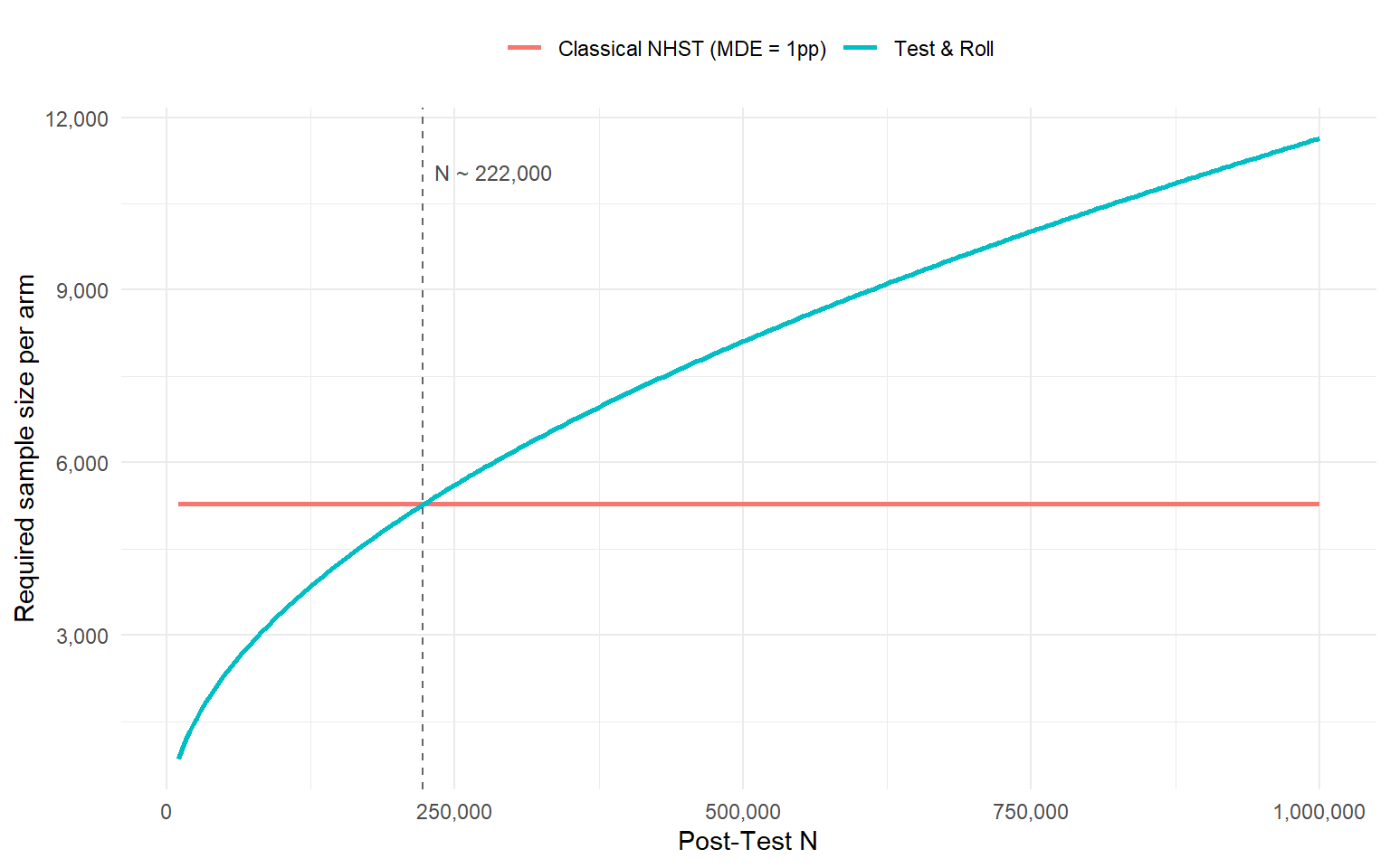
A concrete scenario. Baseline conversion is 3%, the Post-Test population is $N = 500{,}000$, and the lift is believed to follow $\mathcal{N}(0, 0.01^2)$: effects of around one percentage point are typical, most experiments land closer to zero than that. With $s = \sqrt{0.03 \cdot 0.97} \approx 0.171$ and $\sigma_\delta = 0.01$, the formula above returns $n^* \approx 8{,}104$ users per arm. A classical power calculation aimed at the same effect size (`pwr.2p.test()` with `h = ES.h(0.03, 0.04)`, $\alpha = 0.05$, power $= 0.80$) asks for about 5,276 users per arm.
That comparison runs the opposite direction from the one this kind of post usually promises, and it is worth sitting with rather than rounding away. At $N = 500{,}000$, Test & Roll wants *more* data than NHST, not less. The reason is not that Test & Roll has become conservative. It is that $n^*$ grows with $N$ (it scales roughly as $\sqrt{N}$), while the NHST sample size, fixed once you pick an MDE, does not depend on $N$ at all. Run the numbers across a range of $N$ and the two curves cross at roughly $N \approx 223{,}000$. Below that, Test & Roll recommends the dramatically smaller test you would expect; above it, the value at stake in the roll stage (half a million deployments riding on a one-point distinction) makes the extra precision worth paying for. NHST cannot see this because its formula has no $N$ in it. That blindness, not a fixed direction of bias, is the actual lesson, and it is exactly the point made in Section II: the optimal $n$ depends on $N$, and a method that ignores $N$ entirely cannot be calibrated to it in either direction.
Where that crossover sits is scenario-specific, not universal. Feit and Berman's own applications make the point: in their display advertising example, the response is far noisier relative to the typical effect than in the scenario above, and Test & Roll stays an order of magnitude smaller than the NHST benchmark even out to $N = 10^7$. The direction of the comparison depends on how your particular $s$, $\sigma_\delta$, and chosen MDE relate to one another, which is itself a reason to compute $n^*$ for your own numbers rather than trust a rule of thumb either way.
The intuition generalizes past this one example. When $\sigma_\delta$ is large (your tests tend to produce big winners and big losers), a small sample is enough to tell them apart, so $n^*$ stays small regardless of $N$. When effects are small and tightly clustered, as in the scenario above, picking the wrong variant barely costs anything per user, but exactly how little it costs scales with how many users see the decision. NHST has no equivalent of $\sigma_\delta$ to encode either fact. It sizes every test for the same fixed worst case, blind to both the realistic spread of your effects and the size of the population waiting on the other side of the test.
```{r}
#| label: fig-test-roll-vs-nhst
#| fig-cap: "Test & Roll sample size versus the classical NHST sample size, as a function of Post-Test N. The two cross around N ≈ 223,000."
test_roll_n <- function(N, sigma, sigma_delta) {
  # sigma:       within-experiment outcome standard deviation (s in the text)
  # sigma_delta: prior standard deviation of the treatment effect (the lift)
  # Feit & Berman (2019) write the prior on each arm's mean as N(mu, sigma_arm^2);
  # the implied prior on the lift (the difference of two such arms) is
  # N(0, 2 * sigma_arm^2), so sigma_delta^2 = 2 * sigma_arm^2.
  sigma_arm <- sigma_delta / sqrt(2)
  x2 <- (sigma / sigma_arm)^2
  sqrt((N / 4) * x2 + ((3 / 4) * x2)^2) - (3 / 4) * x2
}

N           <- 500000
p0          <- 0.03
sigma       <- sqrt(p0 * (1 - p0))   # within-experiment SD for a binary outcome
sigma_delta <- 0.01

n_star <- test_roll_n(N, sigma, sigma_delta)
n_star
h      <- ES.h(p1 = 0.03, p2 = 0.04)
n_nhst <- pwr.2p.test(h = h, sig.level = 0.05, power = 0.80)$n
n_nhst
N_seq      <- seq(10000, 1000000, length.out = 300)
n_star_seq <- test_roll_n(N_seq, sigma, sigma_delta)
crossover  <- N_seq[which.min(abs(n_star_seq - n_nhst))]

plot_df <- data.frame(
  N      = rep(N_seq, 2),
  n      = c(n_star_seq, rep(n_nhst, length(N_seq))),
  method = rep(c("Test & Roll", "Classical NHST (MDE = 1pp)"), each = length(N_seq))
)

ggplot(plot_df, aes(x = N, y = n, color = method)) +
  geom_line(linewidth = 1) +
  geom_vline(xintercept = crossover, linetype = "dashed", color = "grey40") +
  annotate("text", x = crossover, y = max(plot_df$n) * 0.95,
           label = paste0("N ~ ", format(round(crossover, -3), big.mark = ",")),
           hjust = -0.1, size = 3.2, color = "grey30") +
  scale_x_continuous(labels = scales::comma) +
  scale_y_continuous(labels = scales::comma) +
  labs(x = "Post-Test N", y = "Required sample size per arm", color = NULL) +
  theme_minimal() +
  theme(legend.position = "top")
```
The formula above tells you how large to make the test before it starts. But it commits you to a fixed horizon. What if you want to stop the moment you have enough information to decide, rather than waiting for a pre-registered $n^*$ to fill up? That calls for a different tool: simulation.
## Section IV. The Optimal Stopping Rule: A Simulation Approach
A fixed-horizon test, sized correctly with the formula above, is still a blunt instrument. Some experiments produce a clear signal in the first few days, because the true effect happens to be large; others stay ambiguous for the whole planned duration, because it does not. Committing to $n^*$ in advance means treating both cases identically: you wait out the full test even when the data told you the answer on day four, and you stop at the same moment even when the data is genuinely still unclear. A stopping rule asks a sharper, ongoing question instead: given what has accumulated so far today, is there enough information to act, or is the remaining roll-stage value still worth waiting for? The answer depends on how much value is sitting in the roll stage, which depends on Post-Test $N$, exactly as it did in Section III.
Following the simulation framework in Zaliznyak and Powers (2026, an online technical essay rather than a peer-reviewed paper), we answer this question by simulation, because no closed form exists for the optimal $\theta^*$ the way one exists for $n^*$ in Section III. The two problems differ enough that this is not a small gap to fill. The sample size formula has a clean analytical solution because it asks a *static* question: what $n$ maximizes expected profit before any data exists. The stopping threshold asks a *dynamic* one: given the data observed so far on a given day, is it worth continuing, and that path-dependent optimization over a realistic prior on effects has no known closed form. Draw a true treatment effect for each of many simulated experiments, with positive and negative effects equally likely and most draws close to zero. Run each one day by day, updating the Bayesian posterior on each variant's conversion rate as the data accumulates (updating the Beta-Binomial posterior as in the A/B testing guide). On each day, check whether either variant's $\Pr(\text{best})$ has crossed a candidate threshold $\theta$. The expected loss framework from the A/B testing guide applies here directly: $\Pr(\text{best})$ is exactly the quantity that framework is built around, just tracked day by day instead of computed once at a fixed endpoint. If the threshold is crossed, the experiment stops and deploys the leading variant. Score each candidate $\theta$ by the average long-run value it produces across all simulated experiments, where long-run value is the output captured during the test plus whatever the deployed variant goes on to produce across the rest of $N$. The optimal $\theta^*$ is whichever threshold maximizes that average.
### The θ trap
$\theta^*$ is not a universal constant. It is calibrated to a specific Post-Test $N$ and a specific prior on effect sizes, exactly the two inputs that drove the sample size formula in Section III. Adopting $\theta^* = 0.95$ as a house standard and applying it to every experiment regardless of audience size is precisely the same mistake as $\alpha = 0.05$: a fixed threshold borrowed from someone else's decision problem, not derived from yours.
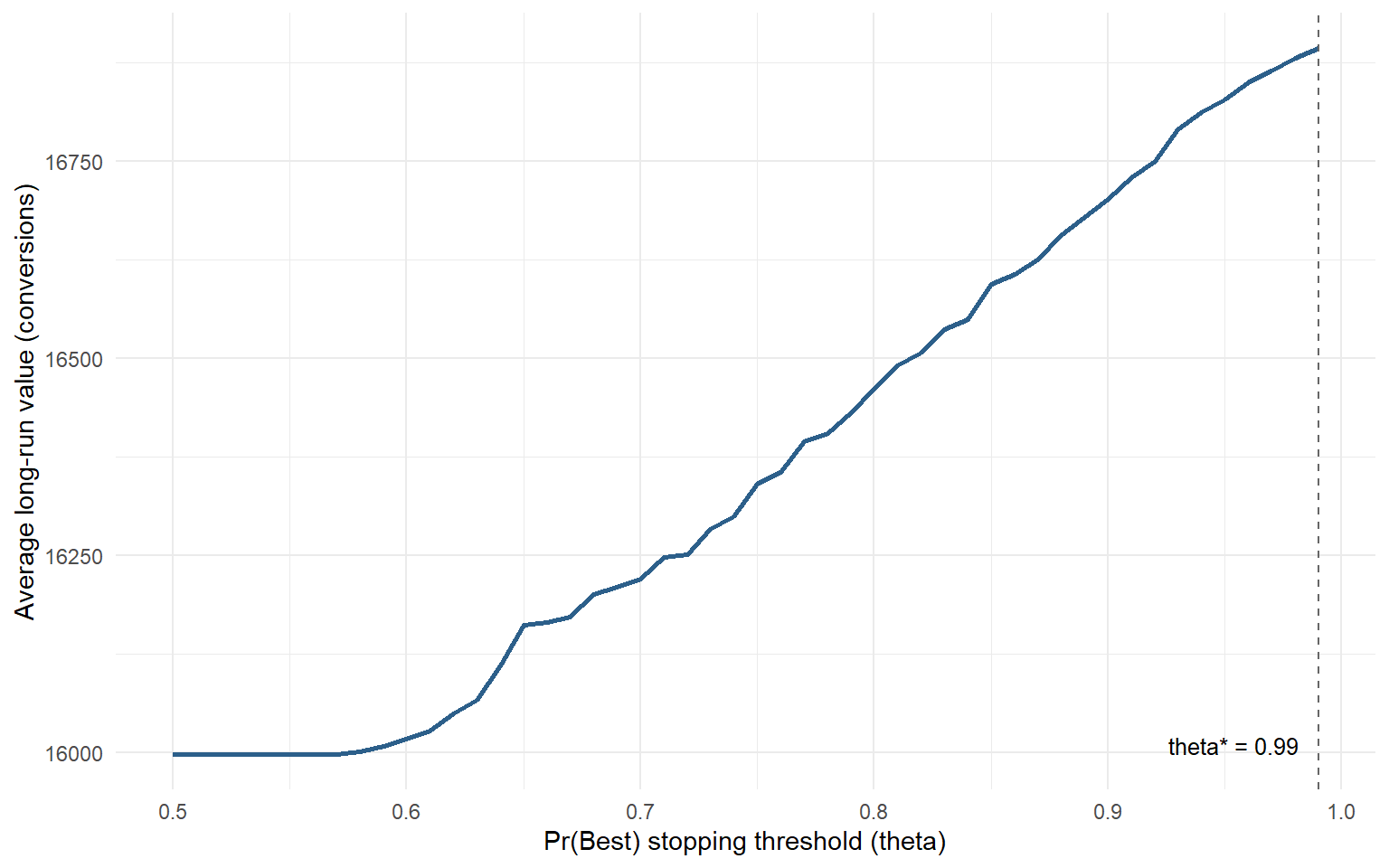
Run this simulation for the same scenario as Section III (baseline conversion 3%, lift $\sim \mathcal{N}(0, 0.01^2)$) and the picture that emerges is a curve that climbs steadily as $\theta$ rises, then flattens. Lower thresholds stop fast but deploy the wrong variant often enough to leave real value on the table; pushing $\theta$ higher buys a steady reduction in error at the cost of a longer test, and for this scenario that trade keeps paying off all the way to the edge of a sensible search range. For $N = 500{,}000$, the curve peaks at $\theta^* = 0.99$: at that threshold, the simulated tests stop after roughly 33 days on average and deploy the wrong variant about 9% of the time, against a roughly threefold higher error rate for thresholds around 0.80. Worth noting for anyone tempted to treat the third decimal as gospel: the curve is nearly flat for $\theta$ above 0.95, so the exact peak matters far less than simply being somewhere in that neighborhood rather than down near 0.80.
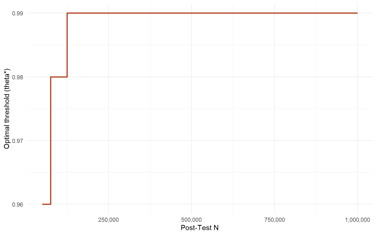
How does $\theta^*$ move with Post-Test $N$? As $N$ grows, so does the value riding on getting the call right, since that one decision gets multiplied across more deployments. The simulation bears this out directly: $\theta^*$ rises from $0.93$ at $N = 50{,}000$ to $0.97$ by $N = 200{,}000$ and reaches $0.99$, the most patient threshold in the grid, by around $N = 350{,}000$, holding there through $N = 10^6$. This mirrors the pattern reported in Zaliznyak and Powers's own simulations: as Post-Test $N$ grows, the stakes of each stopping decision rise, and the optimal threshold rises with them, demanding stronger evidence before committing. There is no dip back down at the largest populations in this scenario. The pull toward patience simply gets stronger and then saturates once the candidate thresholds run out.
```{r}
#| label: run-stopping-simulation
run_simulation <- function(n_sim = 10000, p0 = 0.03, sigma_delta = 0.01,
                            daily_n = 135, max_days = 60,
                            thetas = seq(0.50, 0.99, by = 0.01),
                            seed = 2026) {
  set.seed(seed)
  delta        <- rnorm(n_sim, mean = 0, sd = sigma_delta)
  p_treat_true <- pmin(pmax(p0 + delta, 0.0005), 0.9995)
  p_ctrl_true  <- rep(p0, n_sim)

  stop_day      <- matrix(max_days, nrow = n_sim, ncol = length(thetas))
  deployed      <- matrix(1L,       nrow = n_sim, ncol = length(thetas))
  still_running <- matrix(TRUE,     nrow = n_sim, ncol = length(thetas))

  sC <- rep(0, n_sim); nC <- rep(0, n_sim)
  sT <- rep(0, n_sim); nT <- rep(0, n_sim)
  arm_best <- rep(1L, n_sim)

  # Beta(1, 1) uniform prior on each arm's conversion rate.
  # After s successes in n trials, the posterior is Beta(1 + s, 1 + n - s).
  for (day in seq_len(max_days)) {
    sC <- sC + rbinom(n_sim, daily_n, p_ctrl_true); nC <- nC + daily_n
    sT <- sT + rbinom(n_sim, daily_n, p_treat_true); nT <- nT + daily_n

    aC <- 1 + sC; bC <- 1 + nC - sC
    aT <- 1 + sT; bT <- 1 + nT - sT

    muC  <- aC / (aC + bC);  muT  <- aT / (aT + bT)
    varC <- aC * bC / ((aC + bC)^2 * (aC + bC + 1))
    varT <- aT * bT / ((aT + bT)^2 * (aT + bT + 1))

    # Pr(treatment is best), via the normal approximation to the Beta posteriors
    z         <- (muT - muC) / sqrt(varT + varC)
    pr_t_best <- pnorm(z)
    pr_best   <- pmax(pr_t_best, 1 - pr_t_best)
    arm_best  <- ifelse(muT > muC, 2L, 1L)

    for (j in seq_along(thetas)) {
      crossed <- still_running[, j] & (pr_best > thetas[j])
      if (any(crossed)) {
        stop_day[crossed, j]      <- day
        deployed[crossed, j]      <- arm_best[crossed]
        still_running[crossed, j] <- FALSE
      }
    }
    if (!any(still_running)) break
  }

  still_idx <- which(still_running, arr.ind = TRUE)
  if (nrow(still_idx) > 0) deployed[still_idx] <- arm_best[still_idx[, 1]]

  list(thetas = thetas, stop_day = stop_day, deployed = deployed,
       p_ctrl_true = p_ctrl_true, p_treat_true = p_treat_true,
       daily_n = daily_n)
}

sim <- run_simulation()
```
```{r}
#| label: fig-stopping-results
#| fig-cap:
#| - "Average long-run value by stopping threshold, Post-Test N = 500,000."
#| - "Optimal threshold θ* as Post-Test N varies from 50,000 to 1,000,000."
#| layout-ncol: 2
value_curve <- function(sim, N) {
  sapply(seq_along(sim$thetas), function(j) {
    n_used   <- sim$stop_day[, j] * sim$daily_n * 2
    mu_dep   <- ifelse(sim$deployed[, j] == 2, sim$p_treat_true, sim$p_ctrl_true)
    test_val <- sim$stop_day[, j] * sim$daily_n * (sim$p_ctrl_true + sim$p_treat_true)
    roll_val <- pmax(N - n_used, 0) * mu_dep
    mean(test_val + roll_val)
  })
}

# Panel 1: optimization curve at the worked-example Post-Test N
N_focal    <- 500000
vals       <- value_curve(sim, N_focal)
theta_star <- sim$thetas[which.max(vals)]
curve_df   <- data.frame(theta = sim$thetas, value = vals)

ggplot(curve_df, aes(theta, value)) +
  geom_line(color = "#2C5F8A", linewidth = 1) +
  geom_vline(xintercept = theta_star, linetype = "dashed", color = "grey40") +
  annotate("text", x = theta_star, y = min(curve_df$value),
           label = paste0("theta* = ", theta_star), hjust = 1.15, vjust = 0, size = 3.4) +
  labs(x = "Pr(Best) stopping threshold (theta)",
       y = "Average long-run value (conversions)") +
  theme_minimal()

# Panel 2: how theta* shifts with Post-Test N
N_grid         <- seq(50000, 1000000, by = 25000)
theta_star_seq <- sapply(N_grid, function(N) sim$thetas[which.max(value_curve(sim, N))])
shift_df       <- data.frame(N = N_grid, theta_star = theta_star_seq)

ggplot(shift_df, aes(N, theta_star)) +
  geom_step(color = "#B5482A", linewidth = 1) +
  scale_x_continuous(labels = scales::comma) +
  labs(x = "Post-Test N", y = "Optimal threshold (theta*)") +
  theme_minimal()
```
The practical output of all of this is a single number. Your experimentation platform does not need a p-value, and it does not need an arbitrary 14-day window. It needs $\theta^*$, calibrated once to your typical Post-Test $N$ and your historical effect size distribution, and then a standing rule: stop when $\Pr(\text{best}) > \theta^*$, deploy whichever variant is leading, move on. This also sidesteps the peeking problem documented in Johari et al. (2017): checking a p-value every day and stopping the first time it crosses 0.05 inflates the false positive rate, because every unplanned look is an unaccounted chance to stop on noise. A $\Pr(\text{best})$ threshold does not have that problem, since it is calibrated against a simulation that already includes a look every single day.
Stopping at the right moment solves the question of *when*. It says nothing about whether the effect you measured at that moment is the effect you will actually get once the variant is rolled out. Conditioning on having just crossed a threshold means conditioning on having seen an unusually favorable run of data, and that inflation has a name. It is the Winner's Curse, and it is the subject of Section V.
## Section V. Why the Effect You Shipped Is Probably Too Large
The first two failure modes of NHST-based experimentation live in the design phase: the wrong sample size (Section III) and the wrong stopping rule (Section IV). The third failure happens *after* the test ends, and it does not require you to make a mistake. Even with the right sample size and a flawless stopping rule, the effect you report is still, on average, too large. This is the Winner's Curse.
The name comes from auction theory, and the parallel is exact. In a first-price auction, the winning bid tends to overpay precisely because it was the highest of many noisy guesses about an asset's true value. In experimentation, the bid is your effect-size estimate, the auction is statistical significance, and the asset is the truth. You only "win" (ship a result) when your estimate is unusually large relative to the noise, and that same property that let it win is the property that makes it overpay.
Put more mechanically: when you select results based on statistical significance, you are running a filter that only passes experiments where the observed effect was unusually large. This is not randomness, it is a systematic selection effect. The threshold acts as a floor on the observed effect size. Everything below that floor is invisible to you. Everything above it gets shipped.
Let $\hat{\tau}$ denote the observed treatment effect, $\tau$ the true effect, and SE the standard error of the estimate. Under NHST, you observe and act on $\hat{\tau}$ only when
$$
|\hat{\tau}| > z_{\alpha/2} \cdot \text{SE}
$$
The conditional expectation
$$
\mathbb{E}\big[\hat{\tau} \mid |\hat{\tau}| > z_{\alpha/2} \cdot \text{SE}\big]
$$
is strictly larger in magnitude than $\tau$ whenever power is less than 1. This is the Winner's Curse stated formally. Gelman and Carlin (2014) name the gap between the two quantities the *Type M (magnitude) error*, or *exaggeration ratio*.
### Seeing it in simulation
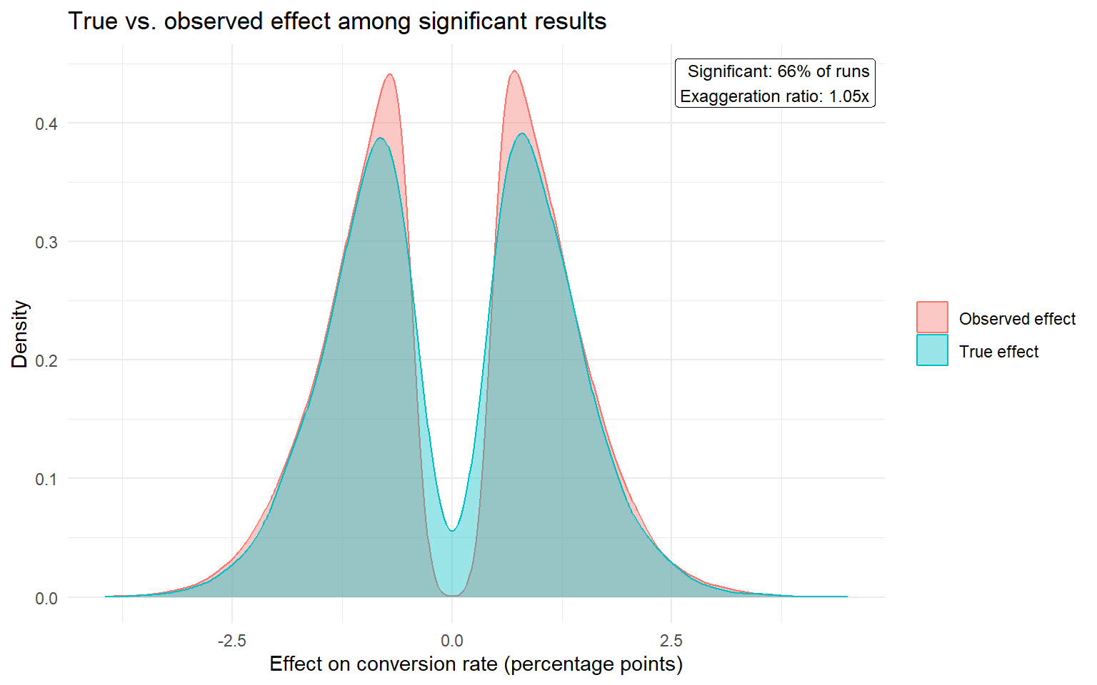
Building on Gelman and Carlin (2014) and using the simulation setup popularised by Zaliznyak (2026, an online technical essay): baseline conversion at 65%, true lifts drawn from $\mathcal{N}(0, 0.01^2)$ so that effects are centred on zero, most small and a few large in either direction, with the design calibrated to detect a 1% relative lift (65% to 65.65%) at 80% power and $\alpha = 0.05$. We reproduce that setup below, drawing 50,000 true effects, simulating a two-sample proportion test for each, and comparing the distribution of true effects against observed effects among the results that reach significance.
```{r}
#| label: fig-winners-curse
#| fig-cap: "True vs. observed effect among statistically significant results. The annotation reports the exaggeration ratio computed in this run."
set.seed(2026)

# Design, calibrated to detect a 1% relative lift at 80% power, alpha = 0.05
baseline <- 0.65
mde_rel  <- 0.01
mde_abs  <- baseline * mde_rel          # 65% -> 65.65%
alpha    <- 0.05
power    <- 0.80
z_alpha  <- qnorm(1 - alpha / 2)
z_beta   <- qnorm(power)

p1 <- baseline
p2 <- baseline + mde_abs
n_per_arm <- ceiling(
  (z_alpha + z_beta)^2 * (p1 * (1 - p1) + p2 * (1 - p2)) / mde_abs^2
)

n_sims      <- 50000
sigma_delta <- 0.01                     # delta ~ N(0, 0.01^2)

true_delta <- rnorm(n_sims, mean = 0, sd = sigma_delta)
treat_rate <- pmin(pmax(baseline + true_delta, 0), 1)

ctrl_successes  <- rbinom(n_sims, n_per_arm, baseline)
treat_successes <- rbinom(n_sims, n_per_arm, treat_rate)

p1_hat  <- ctrl_successes / n_per_arm
p2_hat  <- treat_successes / n_per_arm
tau_hat <- p2_hat - p1_hat
se_hat  <- sqrt(p1_hat * (1 - p1_hat) / n_per_arm + p2_hat * (1 - p2_hat) / n_per_arm)

is_significant <- abs(tau_hat / se_hat) > z_alpha
delta_sig <- true_delta[is_significant]
tau_sig   <- tau_hat[is_significant]

exaggeration <- mean(abs(tau_sig)) / mean(abs(delta_sig))

plot_df <- data.frame(
  effect = 100 * c(delta_sig, tau_sig),
  type   = rep(c("True effect", "Observed effect"), each = length(delta_sig))
)

ggplot(plot_df, aes(x = effect, fill = type, colour = type)) +
  geom_density(alpha = 0.4) +
  annotate(
    "label", x = Inf, y = Inf, hjust = 1.05, vjust = 1.3, size = 3.2, fill = "white",
    label = paste0(
      "Significant: ", round(100 * mean(is_significant)), "% of runs\n",
      "Exaggeration ratio: ", round(exaggeration, 2), "x"
    )
  ) +
  labs(
    x = "Effect on conversion rate (percentage points)", y = "Density",
    title = "True vs. observed effect among significant results",
    fill = NULL, colour = NULL
  ) +
  theme_minimal()
```
The gap between the two densities in the figure is the Winner's Curse, rendered visually. The true-effect distribution among significant results is wide, because almost any true effect, large or small, can occasionally produce a significant draw. The observed-effect distribution sits further from zero, because the only way a small true effect clears the bar is if noise pushed the estimate past it.
### How large is the bias, really
It is tempting to attach a single number to this and move on, but the honest answer depends on power, and the two cleanest numbers worth remembering both come from the original sources rather than from any one simulation run. Running Gelman and Carlin's (2014) own `retrodesign` logic at the power levels practitioners actually argue about: at 80% power the average exaggeration ratio is about 1.12x, at 50% power it is about 1.41x, and you need power to fall to roughly 25% before the ratio crosses 2x, the point at which the shipped effect is, on average, double the truth.
There is a second, complementary way to see the same bias. As shown in Zaliznyak (2026), because the sampling distribution of $\hat{\tau}$ is symmetric around $\tau$, the probability that a significant result overstates the true effect is
$$
\Pr\big(\hat{\tau} > \tau \mid \text{significant}\big) = \frac{0.5}{\text{power}}
$$
At 80% power that is 62.5%, meaningfully more likely to overstate than understate. Below 50% power, the formula's numerator exceeds its denominator, and a significant result is mathematically guaranteed to overstate the true effect, every time.
If your team sizes experiments for fixed two-week windows regardless of expected effect size, you are very likely running below 80% power on a meaningful share of your tests. Below 50% power, a statistically significant result is not merely likely to overstate the truth, it is mathematically guaranteed to. The Winner's Curse is not a statistical curiosity; it is a systematic, predictable overstatement built into every "win" on your roadmap.
This is precisely the Type M error introduced in the [A/B testing guide](https://joaovieira22.github.io/posts/AB%20Testing/ab_test_probably_wrong.html), and now we can see exactly where it comes from mechanically: it is the arithmetic consequence of conditioning on a threshold.
The bias is worse in domains where the true effect distribution has fat tails, such as pricing algorithms or ranking models. Azevedo et al. (2020) estimate a tail coefficient around 1.3 for Bing's core success metric, well below the threshold of 3 that separates thin- from fat-tailed regimes, and find that the top 2% of tested ideas account for roughly 75% of historical gains. When the underlying distribution is this skewed, the significance threshold clips a larger share of the true-effect mass than it would under a normal prior, and the resulting selection effect is correspondingly more severe.
## Section VI. The Fix: Shrink Your Estimates Before You Ship
Two levers fix the Winner's Curse. The first is more power. The second is a prior.
**Increase power.** This works, but it is not free. Holding the minimum detectable effect and significance level fixed, moving from 50% power to 80% power requires the sample size to grow by a factor of $\left(\frac{z_{\alpha/2} + z_{0.80}}{z_{\alpha/2} + z_{0.50}}\right)^2$. With $\alpha = 0.05$ two-sided, $z_{\alpha/2} \approx 1.96$ and $z_{0.80} \approx 0.84$ at 80% power, giving $\left(\frac{1.96 + 0.84}{1.96 + 0}\right)^2 \approx 2.04$. Roughly double the traffic, not the smaller cost some practitioners assume, but nowhere close to free.
**Shrink the estimate.** This is free, requires no additional traffic, and can be applied after the experiment has already ended. It is the focus of the rest of this section.
### The mechanism
You observed $\hat{\tau}$ with standard error SE. You also have a prior over effect sizes, $\mathcal{N}(0, \sigma_\delta^2)$, encoding your belief about how large effects in this domain realistically get. This is the same $\sigma_\delta$ from the Test & Roll formula in Section III, not a new object, just a new use for it. Combining a Gaussian prior with a Gaussian likelihood gives a posterior mean of
$$
\tilde{\tau} = \frac{\sigma_\delta^2}{\sigma_\delta^2 + \text{SE}^2} \cdot \hat{\tau}
$$
This is the shrinkage estimator. When $\sigma_\delta$ is small relative to SE (effects in this domain are usually small and your estimate is noisy), the posterior pulls hard toward zero. When $\sigma_\delta$ is large relative to SE, the posterior barely moves from $\hat{\tau}$.
### A worked example
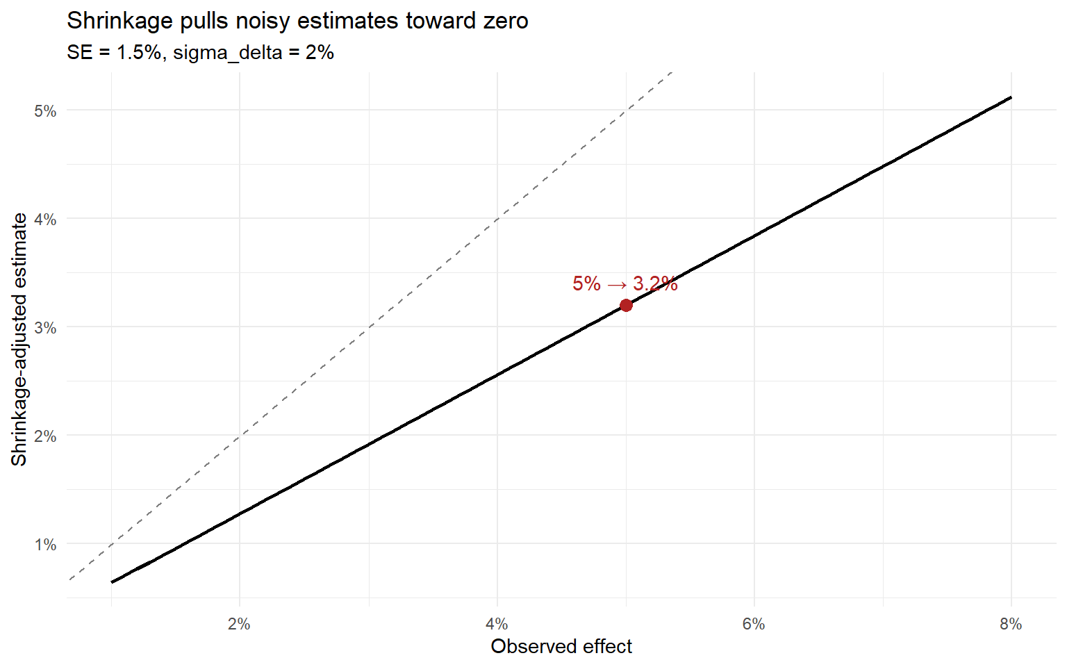
Suppose you observe $\hat{\tau} = 0.05$, with a prior standard deviation on effects of $\sigma_\delta = 0.02$ (you expect most real effects in this domain to fall within about $\pm 4\%$) and a standard error of $\text{SE} = 0.015$. The posterior mean is
$$
\tilde{\tau} = \frac{0.02^2}{0.02^2 + 0.015^2} \cdot 0.05 = \frac{0.0004}{0.000625} \cdot 0.05 \approx 0.64 \times 0.05 = 3.2\%
$$
The shrinkage estimator pulls the reported effect from 5% down to 3.2%. This is not pessimism, it is the correct posterior expectation given a realistic prior on effect sizes. Report 3.2%, not 5%.
```{r}
#| label: fig-shrinkage-curve
#| fig-cap: "Observed effect vs. shrinkage-adjusted estimate. The dashed line marks no shrinkage."
shrink_estimate <- function(tau_hat, se, sigma_delta) {
  (sigma_delta^2 / (sigma_delta^2 + se^2)) * tau_hat
}

se_fixed    <- 0.015
sigma_delta <- 0.02

tau_grid    <- seq(0.01, 0.08, by = 0.001)
tau_shrunk  <- shrink_estimate(tau_grid, se_fixed, sigma_delta)

shrink_df <- data.frame(tau_hat = tau_grid, tau_tilde = tau_shrunk)

example_hat   <- 0.05
example_tilde <- shrink_estimate(example_hat, se_fixed, sigma_delta)

ggplot(shrink_df, aes(x = tau_hat, y = tau_tilde)) +
  geom_abline(slope = 1, intercept = 0, linetype = "dashed", colour = "grey50") +
  geom_line(linewidth = 1) +
  annotate("point", x = example_hat, y = example_tilde, colour = "firebrick", size = 3) +
  annotate(
    "text", x = example_hat, y = example_tilde, vjust = -1, colour = "firebrick",
    label = paste0(round(100 * example_hat, 1), "% \u2192 ", round(100 * example_tilde, 1), "%")
  ) +
  scale_x_continuous(labels = scales::percent) +
  scale_y_continuous(labels = scales::percent) +
  labs(
    x = "Observed effect", y = "Shrinkage-adjusted estimate",
    title = "Shrinkage pulls noisy estimates toward zero",
    subtitle = "SE = 1.5%, sigma_delta = 2%"
  ) +
  theme_minimal()
```
### When to shrink, and when to push back on the prior
Shrinkage earns its keep when your platform runs at low power, when the result in front of you is borderline significant, or when you have a defensible historical estimate of $\sigma_\delta$ from past experiments in the same domain. It earns its keep less when you have strong outside evidence the true effect should be large, or when the test was well-powered enough that SE is small relative to $\sigma_\delta$ in the first place, since the posterior barely moves in that regime anyway.
Estimate $\sigma_\delta$ from your own history: take the standard deviation of observed effects across your platform's past significant experiments, then nudge it down slightly, since those historical estimates carry their own Winner's Curse. If you have no history to draw on, $\sigma_\delta = 0.02$ is a reasonable, conservative starting point for most consumer product metrics.
Wrong sample size, wrong stopping rule, inflated estimate: all three failure modes covered so far live *inside* a single experiment. Section VII asks a different question entirely, not how to run one experiment correctly, but how to allocate a finite experimentation budget across many experiments to maximize long-run value.
## Section VII. Small Wins vs Big Swings: Which Strategy Generates More Value?
Every fix so far has targeted a single experiment: size it correctly (Section III), stop it at the right moment (Section IV), and correct the winner's estimate before acting on it (Sections V–VI). None of that touches a prior question, the one that actually decides how much value a quarter of testing creates. A product team walks into the quarter with a fixed pool of $N_{\text{total}}$ total users for experimentation and a fixed deployment audience of size $N_{\text{post}}$. Before it runs a single test, it has already made the choice that matters most: spend that budget on many small, well-understood bets, or on experiments testing larger, riskier ideas?
Define two strategies, both operating inside the Test & Roll framework of Feit and Berman (2019). Each strategy runs $k$ experiments within the same budget $N_{\text{total}}$, so every experiment receives $n = N_{\text{total}}/k$ test-stage users and is evaluated against the same deployment audience $N_{\text{post}}$. The only difference is the prior on the true effect $\delta$ for each experiment.
**Incremental.** True effects are drawn from $\mathcal{N}(0.005, 0.003^2)$. This is the world of copy edits, button colours, and layout tweaks on a mature surface: nearly all effects are positive, variance is low.
**Big Swing.** True effects are drawn from $\mathcal{N}(0, 0.020^2)$. This is the world of ranking-algorithm rewrites, pricing redesigns, and structurally new features: the prior is centred on zero, the variance is high, and outcomes can be substantially positive *or* substantially negative.
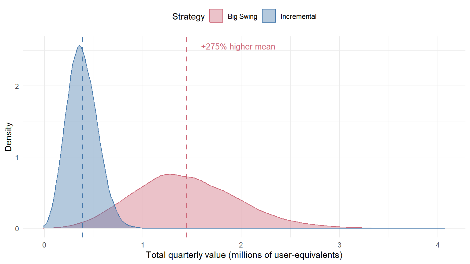
Intuition strongly favours Incremental. Small lifts compound, ship reliably, and rarely produce a bad quarter. The simulation says the opposite: **Big Swings generate roughly 3.8× more average quarterly value than Incremental**, and the mechanism is a direct consequence of a mathematical property that no amount of precision engineering can neutralise.
### The convexity argument
At the end of a test, the roll-stage value of a single experiment is
$$
V(\hat\delta) \;=\; \max(\hat\delta,\; 0)\;\times\; N_{\text{post}},
$$
where $\hat\delta$ is the effect estimate (shrinkage-corrected, per Section VI) and the $\max(\cdot, 0)$ operator encodes the deployment decision: only deploy winners. This function is **convex** in $\hat\delta$, it is flat at zero below the threshold and equal to $\hat\delta \cdot N_{\text{post}}$ above it. Jensen's inequality therefore gives
$$
\mathbb{E}\!\left[V(\delta)\right] \;\geq\; V\!\left(\mathbb{E}[\delta]\right),
$$
with *strict* inequality whenever $\delta$ has positive variance and places mass on both sides of zero. **A wider prior distribution is rewarded, not punished, by a rule that only ever deploys winners.**
The gap is not abstract. For any $\delta \sim \mathcal{N}(\mu, \sigma^2)$, the expected positive part has the closed form
$$
\mathbb{E}[\max(\delta, 0)] \;=\; \mu\,\Phi\!\left(\frac{\mu}{\sigma}\right) \;+\; \sigma\,\phi\!\left(\frac{\mu}{\sigma}\right).
$$
Applying this to the two priors:
| Quantity | Incremental $\mathcal{N}(0.005, 0.003^2)$ | Big Swing $\mathcal{N}(0, 0.020^2)$ |
|---|---|---|
| $\mu$ | 0.005 | 0.000 |
| $\sigma$ | 0.003 | 0.020 |
| $\mathbb{E}[\max(\delta, 0)]$ | ~0.00506 | ~0.00798 |
| Jensen gap vs $\max(\mu, 0)$ | ~0.00006 (tiny) | ~0.00798 (all of it) |
Incremental's option value is almost entirely its mean; the Jensen gap is negligible. Big Swing's option value is *entirely* convexity: its mean is zero, yet it generates a **57.7% higher expected payoff** per deployed experiment than Incremental, before any data are collected.
You only deploy winners. A failed experiment costs you the test-stage traffic and nothing more, the stopping rule prevents you from rolling a loser. A successful experiment is deployed to the full $N_{\text{post}}$. When $N_{\text{post}}$ is large, variance stops being a risk to manage and becomes an asset to seek: the decision rule captures the full upside of a wide prior while truncating its downside at zero.
### Why the gap in practice is far larger than 57.7%
The closed-form ratio of 1.577× assumes the deployment filter is perfect: we always know which experiments have $\delta > 0$ and deploy exactly those. In practice, we deploy when the z-score $\hat\delta / \widehat{\mathrm{se}}$ exceeds the threshold $\theta^*$ (here $\theta^* = 1.96$), using a noisy estimate. This introduces a second, decisive asymmetry.
The detection threshold in effect-size units is $c = \theta^* \times \widehat{\mathrm{se}}$. With $n = 50{,}000$ users per arm and per-user noise $\sigma_y = 0.466$:
$$
\widehat{\mathrm{se}} \;=\; \frac{2\sigma_y}{\sqrt{n}} \;=\; \frac{2 \times 0.466}{\sqrt{50{,}000}} \;\approx\; 0.00417, \qquad c \;=\; 1.96 \times 0.00417 \;\approx\; 0.00817.
$$
For **Incremental**, most true effects ($\mu = 0.005$) lie *below* $c \approx 0.00817$. A given experiment's estimate must be lucky enough to exceed the threshold, an event that happens roughly 27% of the time. Many genuinely positive experiments are *never detected* and their value is never captured. The overall filter efficiency, the fraction of perfect-information value that the filter actually delivers, is only **38%** for Incremental.
For **Big Swing**, effects that exist are large ($\sigma = 0.020$). When a truly large positive effect is present, the threshold is easily crossed. Roughly half of experiments draw a negative true effect and are correctly *not deployed* (the false-positive rate is below 2%). The filter efficiency is **90%** for Big Swing.
| Quantity | Incremental | Big Swing |
|---|---|---|
| $\mathbb{E}[\max(\delta, 0)]$ per experiment | ~0.00506 | ~0.00798 |
| Filter efficiency (fraction captured) | **38%** | **90%** |
| $\mathbb{E}[\delta_{\text{deployed}}]$ per experiment | ~0.00192 | ~0.00722 |
| **Ratio (per experiment)** | | **3.76×** |
The total predicted quarterly value is $k \times \mathbb{E}[\delta_{\text{deployed}} \cdot \mathbf{1}_{\text{deploy}}] \times N_{\text{post}} = 20 \times 0.00192 \times 10^7 \approx 384{,}000$ for Incremental and $\approx 1{,}444{,}000$ for Big Swing. The simulation confirms this.
### Simulation
```{r}
#| label: sim-setup
#| cache: true
set.seed(2026)

# Parameters (matched to Feit & Berman, 2019, website application)
N_total    <- 1e6      # quarterly test-stage user budget
N_post     <- 10e6     # deployment-stage audience (decoupled from test budget)
sigma_y    <- 0.466    # per-user response SD (Feit & Berman website estimate: s = 0.466)
k          <- 20       # number of experiments per quarter, SAME for both strategies
theta_star <- 1.96     # deploy threshold: roll out only when z >= theta*

simulate_quarter <- function(effect_mean, effect_sd) {
  n          <- N_total / k
  se         <- 2 * sigma_y / sqrt(n)       # SE of 2-arm mean difference (n/2 per arm)
  delta_true <- rnorm(k, mean = effect_mean, sd = effect_sd)
  delta_hat  <- delta_true + rnorm(k, sd = se)   # noisy estimate of each effect
  deploy     <- (delta_hat / se) >= theta_star   # one-sided z-test: deploy confirmed positives
  # Payoff: realised by the TRUE effect, summed over all k experiments
  sum(delta_true[deploy]) * N_post
}

reps <- 30000
inc_vals <- replicate(reps,
  simulate_quarter(effect_mean = 0.005, effect_sd = 0.003))
big_vals <- replicate(reps,
  simulate_quarter(effect_mean = 0,     effect_sd = 0.020))

quarterly_value <- tibble(
  strategy    = rep(c("Incremental", "Big Swing"), each = reps),
  total_value = c(inc_vals, big_vals)
)
```
```{r}
#| label: sim-summary
#| echo: false
smry <- quarterly_value |>
group_by(strategy) |>
summarise(
mean_val = mean(total_value),
sd_val = sd(total_value),
p50 = median(total_value),
p90 = quantile(total_value, 0.90),
p99 = quantile(total_value, 0.99),
.groups = "drop"
)
inc_mean <- smry$mean_val[smry$strategy == "Incremental"]
big_mean <- smry$mean_val[smry$strategy == "Big Swing"]
inc_p99 <- smry$p99[smry$strategy == "Incremental"]
inc_sd <- smry$sd_val[smry$strategy == "Incremental"]
big_sd <- smry$sd_val[smry$strategy == "Big Swing"]
pct_lift <- 100 * (big_mean / inc_mean - 1)
```
Across `r format(reps, big.mark=",")` simulated quarters, Big Swing generated `r sprintf("%.0f", pct_lift)`% more average quarterly value than Incremental (`r format(round(big_mean), big.mark=",")` versus `r format(round(inc_mean), big.mark=",")` expected user-equivalents), with `r sprintf("%.1f", big_sd/inc_sd)`× the standard deviation. `r sprintf("%.0f", 100*mean(big_vals > inc_p99))`% of Big Swing quarters exceeded Incremental's 99th-percentile outcome (`r format(round(inc_p99), big.mark=",")`). The Big Swing left tail is bounded: on average, the stopping rule correctly screens out `r sprintf("%.1f", 100*mean(big_vals == 0 | big_vals < 0))`% of quarters where no positive experiment was confirmed, costing only the test-stage traffic.
```{r}
#| label: fig-quarterly-value-density
#| fig-cap: >
#| Distribution of total quarterly value across 30,000 simulated quarters.
#| Vertical dashed lines mark strategy means. Both strategies run k = 20
#| experiments on the same budget. The only difference is the prior on delta.
#| The Big Swing distribution has a fat right tail, individual transformational
#| experiments, that the Incremental strategy structurally cannot produce.
#| fig-width: 8
#| fig-height: 4.5
#| echo: false
means_df <- smry |> select(strategy, mean_val)
ggplot(quarterly_value, aes(x = total_value / 1e6, fill = strategy, colour = strategy)) +
geom_density(alpha = 0.40, linewidth = 0.40) +
geom_vline(data = means_df,
aes(xintercept = mean_val / 1e6, colour = strategy),
linetype = "dashed", linewidth = 0.85, show.legend = FALSE) +
annotate("text",
x = big_mean / 1e6 + 0.15,
y = Inf, vjust = 2.0, hjust = 0,
label = sprintf("+%.0f%% higher mean", pct_lift),
size = 3.5, colour = "#CC6677") +
scale_fill_manual(
values = c("Incremental" = "#4477AA", "Big Swing" = "#CC6677")) +
scale_colour_manual(
values = c("Incremental" = "#4477AA", "Big Swing" = "#CC6677")) +
labs(
x = "Total quarterly value (millions of user-equivalents)",
y = "Density",
fill = "Strategy",
colour = "Strategy"
) +
theme_minimal(base_size = 11) +
theme(legend.position = "top")
```
### Two forces, one conclusion
**Force 1: convexity.** The deployment filter passes large positive draws and blocks large negative draws. A wide prior ($\sigma = 0.020$) puts substantial probability on effects of $0.05$ or more; those draws, once deployed to $10^7$ users, generate enormous value on their own. A narrow prior ($\sigma = 0.003$) has essentially no mass above $0.02$; even a uniformly correct deployment decision cannot produce a transformational outcome because the effect distribution has no tail to exploit.
**Force 2: filter efficiency.** Incremental's typical effect of $0.005$ lies *below* the detection threshold $0.00817$. The experiment must get lucky with its noisy estimate to exceed the threshold, meaning roughly 62% of genuinely positive Incremental experiments are never deployed and their value is permanently forfeited. Big Swing effects are large enough, when they exist, that the detection threshold is crossed reliably, making the filter nearly lossless for positive experiments while correctly screening nearly all negative ones.
Together these two forces explain why the simulated lift (~3.76×) is much larger than the pure-convexity prediction (1.577×): the filter actively penalises the thin-tailed prior and actively rewards the fat-tailed one.
### Where each strategy wins
```{r}
#| label: tbl-decision-table
#| tbl-cap: "Portfolio strategy by domain and effect distribution."
#| echo: false
tibble(
Domain = c(
"Incremental UI copy",
"ML ranking / pricing",
"New product features",
"Mature product, low traffic"
),
`Effect distribution` = c(
"Thin tails, small effects",
"Fat tails, large variance",
"Unknown, potentially large",
"Thin tails, small N_post"
),
`Optimal strategy` = c(
"Incremental",
"Big Swings",
"Big Swings",
"Incremental"
)
) |>
knitr::kable(align = "lll")
```
The pattern in @tbl-decision-table is the practical projection of Azevedo, Deng, Montiel-Olea, Rao, and Weyl (2020), who measured the prior distribution of innovation quality directly from Microsoft Bing's EXP platform. Their headline finding: the tail coefficient of the success-rate metric is $\alpha = 1.31$, far below the critical threshold $\alpha = 3$ at which their Theorem 2 says lean, many-shots experimentation dominates high-powered, few-shot experimentation. Rejections of $\alpha = 2$ and $\alpha = 3$ both carry $p < 0.001$. Empirically, the top 2% of ideas accounted for 74.8% of all historical gains, an extreme Pareto concentration that arises directly from the fat-tailed prior interacting with the deployment filter. The implication is the one this section's simulation produces from first principles: when the tail is fat, the optimal strategy is to maximise shots at it, not to power each shot precisely.
The two analyses are complementary. Azevedo et al. establish *which domains* have fat-tailed priors (search ranking, ad algorithms, pricing); the convexity argument here establishes *why* high prior variance pays regardless of domain, because any one-sided deployment filter creates the asymmetric payoff that Jensen's inequality rewards.
If your effect-size prior has a standard deviation below 1% and your $N_{\text{post}}$ is under 100,000, you are in Incremental territory. If your prior SD exceeds 2% **or** $N_{\text{post}}$ exceeds 500,000, Big Swings dominate. When the two signals point in opposite directions, run the simulation in this section with your own `effect_mean`, `effect_sd`, and `N_post`.
### A concrete recommendation
For teams running ML, pricing, or ranking experiments, where effect distributions tend to be genuinely fat-tailed, default to Big Swings. Size each test to detect an effect two to three times larger than you would target for a UI test, and accept more uncertainty per experiment in exchange for more exposure to the positive tail. The stopping rule from Section IV will protect you from rolling losers; the convexity of the payoff will reward you for the occasional home run.
For copy tests and UI polish on mature, low-traffic surfaces, where the effect distribution is genuinely thin-tailed, Incremental is correct, and precision matters more than variance. The cost of misclassification is asymmetric: applying Incremental logic to a Big Swing domain permanently forfeits the transformational outcomes that dominate long-run value, whereas the reverse mistake merely wastes some test-stage traffic.
Section III fixed the right sample size, Section IV fixed when to stop, Sections V–VI fixed how to correct the estimate, and this section has fixed which portfolio of tests to run. Section VIII pulls all four components into a single R pipeline a practitioner can run end-to-end on a real experiment.
## Section VIII. Full R Implementation: From NHST to Profit-Maximizing Stopping
Sections III through VII each fixed one piece of the experimentation pipeline in isolation: the right sample size, the right stopping rule, the right correction for the Winner's Curse, and the right portfolio of bets to run in the first place. None of that is useful until it runs end to end on one real decision. This section takes a single, concrete test through all four steps, using the same prior structure established throughout the post, $\delta \sim \mathcal{N}(0, \sigma_\delta^2)$, now applied to specific numbers a practitioner could lift directly into their own codebase.
### The scenario
An e-commerce team is testing a change to the checkout flow. Baseline conversion is 3%. The Post-Test population, the number of users who will see the winning variant once the test concludes, is $N = 500{,}000$. The team's prior on the treatment effect is the same one used in Sections III through VII: most checkout tweaks move conversion by a fraction of a point, a few move it more, and the honest starting belief is centred on zero with a standard deviation of one percentage point.
```{r}
#| label: scenario-setup
N           <- 500000   # Post-Test N: population deployed to after the test
p0          <- 0.03     # baseline conversion
sigma_delta <- 0.01     # delta ~ N(0, 0.01^2), the same prior used in Sections III-VII
aov         <- 45       # average order value, EUR, stated assumption for Step 4
```
### Step 1. Sizing the test
`test_roll_n()` from Section III gives the profit-maximizing test size for this $N$, this baseline variance, and this prior. The classical benchmark, sized with `pwr.2p.test()` for the same one-point MDE, gives the comparison.
```{r}
#| label: step1-sizing
n_star <- test_roll_n(N, sqrt(p0 * (1 - p0)), sigma_delta)
n_star
h      <- ES.h(p1 = p0, p2 = p0 + 0.01)
n_nhst <- pwr.2p.test(h = h, sig.level = 0.05, power = 0.80)$n
n_nhst
```
$n^* \approx 8{,}104$ per arm against an NHST benchmark of $n_{\text{NHST}} \approx 5{,}276$. This is the same crossover Section III flagged: at $N = 500{,}000$, above the roughly 223,000 threshold where the two curves cross, Test & Roll asks for *more* data than NHST, not less, because the value sitting in the roll stage is large enough to justify the extra precision. Anyone porting this scenario to a smaller Post-Test $N$ should expect the comparison to flip, exactly as the crossover plot in Section III shows.
### Step 2. Running the test with the optimal stopping rule
Section IV's worked example already calibrated $\theta^*$ for this exact Post-Test $N$, so it does not need to be recomputed here. We extend that section's tooling with one new function, `simulate_single_test()`, which plays out a single realised path of daily data rather than the ten thousand parallel paths `run_simulation()` uses for calibration, and checks the same $\Pr(\text{best}) > \theta^*$ stopping condition each day.
```{r}
#| label: step2-single-test
# Extends Section IV's tooling: simulates ONE realised daily accumulation
# and applies the already-calibrated theta* stopping rule, rather than the
# n_sim parallel paths run_simulation() uses to calibrate theta* itself.
simulate_single_test <- function(p0, sigma_delta, daily_n, max_days, theta_star, seed) {
  set.seed(seed)
  delta_true   <- rnorm(1, mean = 0, sd = sigma_delta)
  p_treat_true <- min(max(p0 + delta_true, 0.0005), 0.9995)
  p_ctrl_true  <- p0

  sC <- 0; nC <- 0; sT <- 0; nT <- 0

  for (day in seq_len(max_days)) {
    sC <- sC + rbinom(1, daily_n, p_ctrl_true); nC <- nC + daily_n
    sT <- sT + rbinom(1, daily_n, p_treat_true); nT <- nT + daily_n

    aC <- 1 + sC; bC <- 1 + nC - sC
    aT <- 1 + sT; bT <- 1 + nT - sT

    muC  <- aC / (aC + bC);  muT  <- aT / (aT + bT)
    varC <- aC * bC / ((aC + bC)^2 * (aC + bC + 1))
    varT <- aT * bT / ((aT + bT)^2 * (aT + bT + 1))

    z         <- (muT - muC) / sqrt(varT + varC)
    pr_t_best <- pnorm(z)
    pr_best   <- max(pr_t_best, 1 - pr_t_best)

    if (pr_best > theta_star) {
      return(list(stop_day = day, tau_hat = sT / nT - sC / nC,
                   se_hat = sqrt(varT + varC), nC = nC, nT = nT,
                   deployed = ifelse(muT > muC, "treatment", "control")))
    }
  }

  list(stop_day = max_days, tau_hat = sT / nT - sC / nC,
       se_hat = sqrt(varT + varC), nC = nC, nT = nT,
       deployed = ifelse((sT / nT) > (sC / nC), "treatment", "control"))
}

# theta_star carries over from Section IV's worked example, which already
# used this exact N = 500,000, so it is not recalibrated here.
result <- simulate_single_test(p0 = p0, sigma_delta = sigma_delta, daily_n = 135,
                                max_days = 60, theta_star = theta_star, seed = 2026)
result$stop_day
result$deployed
```
In this realisation, $\Pr(\text{best})$ never clears $\theta^* = 0.99$ before the planned 60-day window closes; it reaches roughly 0.955 by day 60 without crossing 0.99, the threshold Section IV's value-curve optimisation returns for this $N$. The test runs the full window and is deployed at the day-60 read, since the posterior still favours treatment. That is not a failure of the stopping rule, it is the rule working as intended at this scale: with $N = 500{,}000$ waiting in the roll stage, the value-curve optimisation in Section IV pushes $\theta^*$ close to certainty, because a few extra days of testing cost almost nothing next to the value of being right about which variant reaches half a million users. Worth noting for anyone replicating this: at $135$ users per arm per day, 60 days lands at 8,100 per arm, within four users of the $n^* \approx 8{,}104$ that Step 1 derived independently from the closed-form formula. The fixed-horizon sizing and the calibrated stopping rule agree almost exactly here, which is itself a useful sanity check that the two tools in Sections III and IV are pointing at the same answer.
### Step 3. Correcting for the Winner's Curse
`shrink_estimate()` from Section VI takes the raw effect observed at the stopping day and pulls it toward zero using the same $\sigma_\delta$ prior that has been used throughout.
```{r}
#| label: step3-shrinkage
tau_hat   <- result$tau_hat
se_hat    <- result$se_hat
tau_tilde <- shrink_estimate(tau_hat, se_hat, sigma_delta)
tau_hat
tau_tilde
```
The raw observed effect is roughly $0.42$ percentage points; the shrinkage-adjusted estimate is roughly $0.39$ percentage points. The correction is modest here because 8,100 observations per arm produce a standard error small enough, relative to $\sigma_\delta = 0.01$, that the posterior does not move far from the data. That is not always the case, and Step 4 uses the shrunk number, not the raw one, on principle.
### What changed between the raw and shrinkage-adjusted numbers
The raw observed effect implies roughly €101,112 in incremental revenue; the shrinkage-adjusted effect implies roughly €94,276. Skipping Step 3 overstates the number a VP would see by about 7%, not because the raw estimate is fabricated, but because it is the unconditional expectation of a number that was only reported because it crossed a threshold.
### Step 4. Computing the roll-stage value
The shrinkage-adjusted estimate, not the raw one, feeds the roll-stage calculation: the remaining population times the corrected lift, translated into revenue at an assumed average order value of €45.
```{r}
#| label: step4-revenue
roll_population          <- N - n_star
incremental_conversions  <- roll_population * tau_tilde
incremental_revenue      <- incremental_conversions * aov
roll_population
incremental_conversions
incremental_revenue
```
```{r}
#| label: summary-table
summary_tbl <- data.frame(
  Metric = c("Test & Roll n* (per arm)", "NHST n (per arm)", "Stopping day",
             "Raw observed effect", "Shrinkage-adjusted effect",
             "Expected incremental revenue (EUR)"),
  Value = c(
    format(round(n_star), big.mark = ","),
    format(round(n_nhst), big.mark = ","),
    result$stop_day,
    paste0(round(100 * tau_hat, 3), "%"),
    paste0(round(100 * tau_tilde, 3), "%"),
    paste0("\u20AC", format(round(incremental_revenue), big.mark = ","))
  )
)
knitr::kable(summary_tbl, align = "lr")
```
The pipeline produces a single defensible number: roughly **€94,000** in expected incremental revenue from rolling this checkout change out to the remaining Post-Test population, net of the Winner's Curse correction.
### Step 5. Where this sits in the portfolio
With $N_{\text{post}} \approx 500{,}000$, this test sits almost exactly on the boundary Section VII draws between Incremental and Big Swing territory, closer in spirit to the thin-tailed Incremental example than to the wide Big Swing prior, but running at a Post-Test $N$ large enough to sit right at the edge where Section VII's own classification rule starts to favour wider bets. The honest read is that a single checkout-copy tweak like this one is correctly treated as Incremental: precision matters more here than variance, and the small, defensible revenue number above is exactly the kind of outcome that strategy is built to produce. But a team running only tests shaped like this one, on a surface this large, is leaving the convexity gains from Section VII on the table. The checkout flow is worth the occasional Big Swing test too, a structural redesign rather than a copy change, sized and evaluated with the same pipeline, but drawn from a wider prior.
This pipeline produces a number you can defend to a VP. The final section turns that pipeline into a decision framework: knowing which of these tools is the right one to reach for, and when.
## Section IX. A Decision Framework: When to Use Each Approach
Four tools have been built across this post, and each solves a real problem the others do not. The question a practitioner actually has, standing in front of a new test, is not "which of these is correct?" but "which of these is correct for *this* test?" The table below is built to answer that in under a minute.
| Approach | Best for | Requires | Weakness |
|---|---|---|---|
| Classical NHST | Regulatory or compliance contexts, low Post-Test N, symmetric error costs | A fixed MDE chosen in advance and a pre-registered significance level | Ignores N entirely, treats false positives and false negatives as equally costly when they rarely are, and routinely sizes tests larger or smaller than the decision actually warrants |
| Test & Roll | Most product and growth experiments with a known Post-Test N | A reasonable prior on $\sigma_\delta$, ideally estimated from the historical spread of the team's own past effects | The prior can be wrong, and a badly miscalibrated $\sigma_\delta$ produces a sample size as misleading as the NHST number it was meant to replace |
| mSPRT or always-valid monitoring | Teams that need frequentist Type I error guarantees while peeking continuously | A pre-specified alpha-spending function fixed before the test starts | More conservative than the Bayesian $\Pr(\text{best})$ stopping rule from Section IV, since it is built to control error rates rather than maximise expected value |
| Bayesian expected loss or $\Pr(\text{best})$ stopping | Teams optimising for long-run profit who are comfortable reporting posterior probability statements | A loss function or an explicit business tolerance $\theta$ for how much expected value to leave on the table | Does not control frequentist Type I error without further calibration, which matters if the result will be reported outside the team that ran the test |
These four are not mutually exclusive, and treating them as competing schools of thought misses the point of building all four into one pipeline. As discussed in the A/B testing guide, a mature experimentation programme typically runs NHST or mSPRT at the platform level, for guardrail monitoring across hundreds of simultaneous experiments where frequentist error control genuinely matters, and reserves Test & Roll plus Bayesian stopping for the individual ship-or-hold decision on any one test, where the objective is profit rather than error control. The two layers answer different questions, and a platform that uses only one of them is either over-controlling individual decisions it should be optimising, or under-controlling the aggregate false-positive rate across a portfolio it should be guarding.
### Five questions for your analytics team
**What is our $\sigma_\delta$, and where did it come from?** A team that can answer this with a number pulled from the historical variance of past effects has a calibrated prior. A team that answers with a guess, or with the MDE from a template, is running Test & Roll with NHST's same blind spot, just renamed.
**What is our Post-Test N for this specific test?** If the answer is a formula, sample size was set by the actual economics of the decision. If the answer is "we always run two weeks," sample size was set by habit, and Section III's whole argument is that habit and optimal $n^*$ rarely agree.
**Did we correct for the Winner's Curse before reporting this number?** A reported lift that has not been shrunk is the raw, threshold-conditioned estimate Section V described, not a defensible number. The gap between the two, as Step 3 of Section VIII showed, is rarely zero.
**Is this test an Incremental or a Big Swing, and does our traffic allocation reflect that classification?** A team that cannot answer this is very likely running everything as a cautious Incremental test by default, which Section VII showed forfeits most of the convexity gain available from a wider portfolio.
**What would we have to believe about $\sigma_\delta$ for our current sample size practice to be optimal?** This question runs the logic backward: given the sample sizes the team actually uses, what implicit prior would make that choice optimal? When the implicit answer does not match what the team actually believes about its own effect sizes, the practice is inconsistent with the team's stated beliefs, and that inconsistency is usually costing real revenue.
Statistical significance was built to answer a different question than the one a business needs answered: whether an effect is real, not whether acting on it is worth more than it costs. Test & Roll, optimal stopping, shrinkage correction, and portfolio allocation are not exotic alternatives bolted onto that framework. They are the direct consequence of asking the right question from the start, what allocation of *this* specific budget, to *this* specific population, maximises expected value. Every method in this post follows from that one reframing, and the pipeline in Section VIII is what it looks like applied to a single afternoon's worth of checkout data.
## References
- Azevedo, E. M., Deng, A., Montiel Olea, J. L., Rao, J. M. & Weyl, E. G. (2020). A/B Testing with Fat Tails. *Journal of Political Economy*, 128(12), 4614–4672.
- Feit, E. M. & Berman, R. (2019). Test & Roll: Profit-Maximizing A/B Tests. *Marketing Science*, 38(6), 1038–1058.
- Fisher, R. A. (1925). *Statistical Methods for Research Workers*. Oliver & Boyd.
- Gelman, A. & Carlin, J. (2014). Beyond power calculations: Assessing type S (sign) and type M (magnitude) errors. *Perspectives on Psychological Science*, 9(6), 641–651.
- Gigerenzer, G. (2004). Mindless statistics. *Journal of Socio-Economics*, 33(5), 587–606.
- Hubbard, R. (2004). Alphabet Soup: Blurring the distinctions between p's and α's in psychological research. *Theory & Psychology*, 14(3), 295–327.
- Johari, R., Koomen, P., Pekelis, L. & Walsh, D. (2017). Peeking at A/B Tests: Why it Matters and What to Do About It. *KDD '17*, 1517–1525.
- Kohavi, R., Tang, D. & Xu, Y. (2020). *Trustworthy Online Controlled Experiments: A Practical Guide to A/B Testing*. Cambridge University Press.
- Lindquist, E. F. (1940). *Statistical Analysis in Educational Research*. Houghton Mifflin.
- Neyman, J. & Pearson, E. S. (1933). On the problem of the most efficient tests of statistical hypotheses. *Philosophical Transactions of the Royal Society A*, 231, 289–337.
- Zaliznyak, R. (2025). The Value of Big Swings. *rzaliznyak-math.github.io*. [https://rzaliznyak-math.github.io/main/ab-testing/big-swings.html](https://rzaliznyak-math.github.io/main/ab-testing/big-swings.html)
- Zaliznyak, R. (2026). The Winner's Curse. *rzaliznyak-math.github.io*. [https://rzaliznyak-math.github.io/main/ab-testing/winners-curse.html](https://rzaliznyak-math.github.io/main/ab-testing/winners-curse.html)
- Zaliznyak, R. & Powers, J. (2026). AB Testing is an Optimization Problem. *rzaliznyak-math.github.io*. [https://rzaliznyak-math.github.io/main/ab-testing/ab-testing-optimization.html](https://rzaliznyak-math.github.io/main/ab-testing/ab-testing-optimization.html)